Healthcare costs affect everyone. From routine checkups to major treatments, the bills can add up fast. Insurance companies try to predict these costs so they can set fair premiums. But what if we could also use tools like polynomial regression in machine learning to make medical cost predictions?
That’s exactly what this project is about. Using the Medical Cost Personal Dataset from Kaggle, we’ll explore how factors like age, BMI, smoking habits, and family size influence insurance charges. Our goal is to build regression models that can make reliable predictions about future costs.
This project is part of my learning journey. Earlier, I built a linear regression model with NumPy to predict house prices. Now, we’ll be moving one step further with Scikit-Learn and trying out polynomial regression alongside regularized models like Ridge and Lasso.
By the end of this article, you’ll see how to clean the data, build models, compare their performance, and interpret the results. More importantly, you’ll understand how regression techniques can turn messy real-world data into actionable insights.
Step 1: Importing Libraries
Every machine learning project begins with the right tools. In Python, these tools come as libraries. Each library has a special role, like helping us handle data, run models, or make plots.
For this project, we’ll use:
- NumPy: for math operations and arrays.
- Pandas: for loading and exploring the dataset in table form.
- Matplotlib and Seaborn: for making charts and plots.
- Scikit-Learn: for building and testing regression models.
Here’s the code to bring them in:
# Data manipulation
import numpy as np
import pandas as pd

# Visualizations
import matplotlib.pyplot as plt
import seaborn as sns

# Machine learning tools
import statsmodels.api as sm
from scipy.special import inv_boxcox
from scipy.stats import f_oneway, boxcox
from sklearn.linear_model import LinearRegression, Ridge, Lasso
from sklearn.metrics import r2_score, mean_squared_log_error
from sklearn.model_selection import train_test_split, KFold, GridSearchCV
from sklearn.pipeline import Pipeline
from sklearn.preprocessing import OneHotEncoder, StandardScaler, PolynomialFeaturesWhen I was starting, I found it helpful to think of these imports as a toolbox. Each line gives us access to a set of ready-made functions, so we don’t have to build everything from scratch.
Step 2. Import and Preview the Dataset
Now that we have our tools ready, the next step is to load the dataset and take a first look at what it contains. In this project, we are working with a medical insurance dataset that holds information about people’s age, gender, BMI (Body Mass Index), number of children, smoking status, region, and insurance charges.
2.1 Import Datsset
We start by loading the dataset with pandas and checking out the first few rows:
data = pd.read_csv('medical-insurance.csv')
data.head()
Right away, we can see the dataset is made of seven columns, with the last one (charges) being the target variable we want to predict.
2.2 Checking the dataset details
To better understand the structure, we check the data types and non-null counts:
data.info()RangeIndex: 1338 entries, 0 to 1337
Data columns (total 7 columns):
# Column Non-Null Count Dtype
--- ------ -------------- -----
0 age 1338 non-null int64
1 sex 1338 non-null object
2 bmi 1338 non-null float64
3 children 1338 non-null int64
4 smoker 1338 non-null object
5 region 1338 non-null object
6 charges 1338 non-null float64
dtypes: float64(2), int64(2), object(3)
This tells us:
- We have 1338 rows and 7 columns.
- There are no missing values.
age,bmi,children, andchargesare numeric.sex,smoker, andregionare categorical.
2.3 Previewing categorical variables
Finally, we check the unique categories for the categorical columns:
# Select all categorical columns from the dataset
categorical_vars = data.select_dtypes(include=['object']).columns

# Loop through each categorical column and print its unique values
for col in categorical_vars:
    unique_vals = data[col].unique().tolist()

    print(f'=== {col} ===')
print(unique_vals)=== sex ===
['female', 'male']
=== smoker ===
['yes', 'no']
=== region ===
['southwest', 'southeast', 'northwest', 'northeast']
This confirms that:
sexhas two categories (female, male).smokerhas two categories (yes, no).regionhas four categories (southwest, southeast, northwest, northeast).
Step 3: Data Cleaning
Before we can trust our dataset for modeling, we need to make sure it’s clean. Even small issues like duplicate rows or missing values can affect our model’s performance. Let’s check for these step by step.
3.1 Checking for duplicate rows
Sometimes datasets have duplicate entries, meaning the same record appears more than once. These don’t add value and can bias our model, so we remove them if found.
print(f'Duplicated rows: {data.duplicated().sum()}')Duplicated rows: 1
We see that there’s 1 duplicate row. Let’s drop it:
data = data.drop_duplicates()Now our dataset only contains unique records.
3.2 Checking for missing values
Next, we need to confirm if any values are missing. Missing values can cause errors during training or distort our analysis.
print(f'Missing values: {data.isnull().sum().sum()}')Missing values: 0
Great news, there are no missing values in this dataset.
At this point, our dataset is clean. With duplicates removed and no missing values, we’re ready to move on to exploring and analyzing the data.
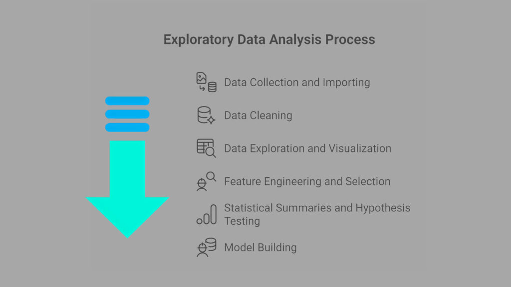
Step 4: Exploratory Data Analysis (EDA) and Hypothesis Testing
Before training any model, we need to understand our data. With Exploratory Data Analysis (EDA), we look at how the variables are distributed, check for outliers, and see how features relate to the target.
Alongside EDA, we use hypothesis testing to answer questions like:
- Do smokers really pay more in medical charges than non-smokers?
- Does age or BMI have a significant effect on costs?
EDA gives us a visual story of the data. Hypothesis tests add statistical evidence to confirm patterns we see. Together, they form the foundation for building reliable models.
4.1 Exploring the Target Variable: Charges
Before building models, we need to understand our target variable, charges. This column shows the total medical expenses billed to each patient.
4.1.1 Charges Distribution
We will begin by plotting its distribution using a histogram and a boxplot.
# Helper function
def plot_numerical_variables(data, col):
    """
    Plots the distribution of numerical variables.
    :param data: (dataframe) dataset
    :param col: (string) column name
    :return: None
    """
    plt.figure(figsize=(14, 5))

    # Histogram
    plt.subplot(1, 2, 1)
    sns.histplot(data[col], kde=True)
    plt.title(f'Distribution of {col.capitalize()}', fontsize=16)
    plt.xlabel(col.capitalize(), fontsize=14)
    plt.ylabel('Count', fontsize=14)

    # Boxplot
    plt.subplot(1, 2, 2)
    sns.boxplot(data[col], color='lightgreen')
    plt.title(f'Boxplot of {col.capitalize()}', fontsize=16)
    plt.ylabel('Count', fontsize=14)
# Plot histogram and boxplot of the tartget variable `charges`
plot_numerical_variables(data=data, col='charges')
The histogram shows us how the values are spread out, while the boxplot highlights possible outliers.
What do we see?
- Most patients have charges between $1,000 and $20,000.
- A few patients are billed far higher, with costs going above $60,000.
- The boxplot confirms the presence of many outliers on the higher end.
4.1.2 Charges Summary Statistics
Next, let’s check the summary statistics:
data['charges'].describe()count 1337.000000
mean 13279.121487
std 12110.359656
min 1121.873900
25% 4746.344000
50% 9386.161300
75% 16657.717450
max 63770.428010
Name: charges, dtype: float64
From these numbers:
- The average charge is ~$13,279, but the standard deviation is almost as high, showing wide variation.
- The median is ~$9,386, which is lower than the mean, hinting at right skewness.
- The maximum charge of $63,770 is much higher than the rest, which explains the outliers.
4.1.3 Charges Outliers and Skew
Finally, let’s confirm skewness and count outliers programmatically:
# Helper function
def outliers_skew(data, col):
    """
    Detects outliers and calculates skewness for a given numerical column.

    Parameters
    ----------
    data : pandas.DataFrame
        The dataset containing the column to check.
    col : str
        The name of the numerical column to analyze.

    Returns
    -------
    None
        Prints the number of outliers and the skewness value.
    """
    # Calculate interquartile range (IQR)
    q1 = data[col].quantile(0.25)
    q3 = data[col].quantile(0.75)
    iqr = q3 - q1

    # Define lower and upper bounds for outliers
    lower = q1 - iqr * 1.5
    upper = q3 + iqr * 1.5

    # Identify outliers
    outliers = data[(data[col] < lower) | (data[col] > upper)][col]

    print(f'Outliers: {len(outliers)}')
    print(f'Skew: {data[col].skew():.2f}')
# Check for outliers and skew
outliers_skew(data=data, col='charges')Outliers: 139
Skew: 1.52
Interpretation:
- The skew value of 1.52 tells us the distribution is positively skewed (a long tail to the right).
- About 139 patients are statistical outliers with very high charges.
This makes sense in real life: most people pay moderate medical costs, but a small group with serious conditions may face huge bills.
4.2 Exploring Categorical Variables
So far, we have looked at the numeric side of the data. Now, let’s switch to the categorical variables:
sex(male or female)smoker(yes or no)region(northeast, northwest, southeast, southwest)
4.2.1 Categorical Distributions
We begin with count plots to see how many patients fall into each category.
# Set number of columns and rows for subplots
n_cols = 3
n_rows = math.ceil(len(categorical_vars) / n_cols)

# Create figure with dynamic size based on number of plots
plt.figure(figsize=(6 * n_cols, 4 * n_rows))

# Loop through each categorical variable and plot its distribution
for i, col in enumerate(categorical_vars, 1):
    plt.subplot(n_rows, n_cols, i)  # Place subplot in grid
    sns.countplot(x=data[col], palette='Set2')  # Bar plot of category counts
    plt.title(f'Distribution of {col.capitalize()}', fontsize=16)
    plt.xlabel(col.capitalize(), fontsize=14)
    plt.ylabel('Count', fontsize=14)

plt.show()
Here is what we find:
- The dataset is balanced between male (50.5%) and female (49.5%).
- Only 20% of patients are smokers, while 80% are non-smokers.
- The four regions are almost evenly represented, each around 24–27%.
This balance is good. It means our model will not be biased toward one group.
4.2.2 Mean Charges by Category
Next, we check the average charges in each category:
# Loop through each categorical variable
for col in categorical_vars:
    # Calculate mean charges for each category in the variable
    average_charges = data.groupby(col)['charges'].mean().to_frame(name='Mean')

    print(f'=== {col} ===')
print(average_charges)=== sex ===
Mean
sex
female 12569.578844
male 13974.998864
=== smoker ===
Mean
smoker
no 8440.660307
yes 32050.231832
=== region ===
Mean
region
northeast 13406.384516
northwest 12450.840844
southeast 14735.411438
southwest 12346.937377
Findings:
Sex: Males pay a little more on average ($13,975) than females ($12,570).Smoker: Smokers pay dramatically more ($32,050) compared to non-smokers ($8,440).Region: Southeast has the highest average charges (~$14,735), while southwest is lowest (~$12,347).
The smoker difference really stands out. Let’s test if this is statistically significant.
4.2.3 Category Hypothesis Testing with ANOVA
We use ANOVA (Analysis of Variance) to check if the mean charges differ between groups.
# ANOVA test for categorical variables against medical charges
alpha = 0.05  # significance level

for col in categorical_vars:
    # Split 'charges' into groups based on the current categorical variable
    groups = [group['charges'] for _, group in data.groupby(col)]

    # Perform one-way ANOVA test
    f_stats, p_value = f_oneway(*groups)

    print(f'=== {col} ===')
    print(f'F-statistic: {f_stats:.2f}, p-value: {p_value:.4e}')
    print(f'Null Hypothesis: Average charges are the same across {col}.')

    # Decision rule based on significance level
    decision = "Reject the null hypothesis." if p_value < alpha else "Fail to reject the null hypothesis."
print(f'Decision: {decision}')=== sex ===
f-stats: 4.51, p-value: 0.033820791995078286
Null Hypothesis: Average charges are the same across sex.
Decision: Reject the null hypothesis.
=== smoker ===
f-stats: 2175.74, p-value: 1.4067220949358597e-282
Null Hypothesis: Average charges are the same across smoker.
Decision: Reject the null hypothesis.
=== region ===
f-stats: 2.93, p-value: 0.03276288025444947
Null Hypothesis: Average charges are the same across region.
Decision: Reject the null hypothesis.
Results:
Sex: p = 0.034 → Reject the null. There is a difference.Smoker: p ≈ 0 → Reject the null strongly. Huge difference in charges.Region: p = 0.033 → Reject the null. Regions differ slightly.
Takeaways
- Being a smoker is the biggest driver of high medical charges.
- Gender and region also have some influence, but the effect is smaller.
- These insights will be important when we build our models.
4.3 Exploring Numerical Variables
Now let’s look at the numerical variables:
age(patient’s age)bmi(body mass index, a measure of body fat)children(number of dependents)
These features may explain why charges vary among patients.
4.3.1 Numerical Summary Statistics
# Select numerical columns (int and float types) from the dataset
numerical_cols = data.select_dtypes(include='number').columns

# Drop the target variable 'charges' so we only analyze predictors
numerical_vars = numerical_cols.drop(['charges'])

# Display descriptive statistics for numerical variables (transpose for readability)
data[numerical_vars].describe().Tcount mean std min 25% 50% 75% max
age 1337.0 39.222139 14.044333 18.00 27.00 39.0 51.0 64.00
bmi 1337.0 30.663452 6.100468 15.96 26.29 30.4 34.7 53.13
children 1337.0 1.095737 1.205571 0.00 0.00 1.0 2.0 5.00
Most patients are around 39 years old, with BMI around 30, and about 1 child on average.
4.3.2 Numerical Distributions
We plot histograms and boxplots for each variable.
# Loop through each numerical variable and plot its distribution
for col in numerical_vars:
    plot_numerical_variables(data=data, col=col)

plt.show()


Observations:
Ageis roughly normally distributed between 18 and 64, with no outliers.BMIhas a small number of outliers on the high side (very high BMI).Childrenis right-skewed, since many patients have 0–1 child, while fewer have 4–5.
4.3.3 Numerical Outliers and Skew
# Check each numerical variable for outliers and skewness
for col in numerical_vars:
    print(f'=== {col} ===')
outliers_skew(data=data, col=col)=== age ===
Outliers: 0
Skew: 0.05
=== bmi ===
Outliers: 9
Skew: 0.28
=== children ===
Outliers: 0
Skew: 0.94
Observations:
Age: 0 outliers, skew = 0.05 (almost symmetric).BMI: 9 outliers, skew = 0.28 (slightly right-skewed).Children: 0 outliers, skew = 0.94 (moderately skewed).
4.3.4 Correlation and Multicollinearity Between Variables
Next, we check correlations to see if variables are strongly related.
# Calculate correlation matrix for numerical variables
corr_mat = data[numerical_vars].corr()

# Keep only the upper triangle of the correlation matrix (to avoid duplicates)
upper_mat = corr_mat.where(np.triu(np.ones(corr_mat.shape), k=1).astype(bool))

# Identify variables with correlation above 0.8 (multicollinearity threshold)
mult_col = [col for col in upper_mat.columns if any(upper_mat[col] > 0.8)]

print(f'Multi-collinear: {len(mult_col)}')Multi-collinear: 0
# Compute correlation matrix including the target variable 'charges'
corr = data[numerical_cols].corr()

# Plot a heatmap to visualize correlations between numerical variables
plt.figure(figsize=(8, 5))
sns.heatmap(corr, annot=True, cmap='coolwarm', linewidths=0.5)

plt.show()
No two numerical variables are highly correlated with each other (so no multicollinearity). But we do see that age and BMI have moderate correlation with charges.
4.3.5 Relationship with Charges
Scatter plots with regression lines give us a visual clue:
# Create a grid of subplots based on number of numerical variables
n_cols = 3
n_rows = math.ceil(len(numerical_vars) / n_cols)
plt.figure(figsize=(6 * n_cols, 4 * n_rows))

# Plot scatterplots for each numerical variable against the target 'charges'
for i, col in enumerate(numerical_vars, 1):
    plt.subplot(n_rows, n_cols, i)

    # Scatterplot shows relationship between the feature and target
    sns.scatterplot(data=data, x=col, y='charges', alpha=0.6)

    # Add a regression line (red) to highlight overall trend
    sns.regplot(data=data, x=col, y='charges', scatter=False, color='red')

    # Add labels and title
    plt.title(f'{col.capitalize()} vs. Charges', fontsize=16)
    plt.xlabel(col.capitalize(), fontsize=14)
    plt.ylabel('Charges', fontsize=14)

plt.show()
Observations:
AgevsCharges: Older patients tend to have higher charges.BMIvsCharges: Higher BMI is linked with higher charges, but the relationship is weaker.ChildrenvsCharges: The number of children has only a small effect.
4.3.6 Hypothesis Tests
We confirm the relationships with hypothesis testing:
# Significance level for hypothesis testing
alpha = 0.05

# Loop through each numerical variable and test its predictive power on charges
for col in numerical_vars:
    x = data[col]            # Feature (independent variable)
    y = data['charges']      # Target (dependent variable)

    # Add constant term (intercept) for the regression model
    x = sm.add_constant(x)

    # Fit an Ordinary Least Squares (OLS) regression model
    model = sm.OLS(y, x).fit()

    # Extract the p-value for the feature
    p_value = model.pvalues[col]

    print(f'=== {col} ===')
    print(f'Null hypothesis: {col} is not a strong predictor of charges.')
    print(f'p-value: {p_value}')

    # Decision rule: reject null hypothesis if p-value < alpha
    decision = 'Reject the null hypothesis.' if p_value < alpha else 'Fail to reject the null hypothesis.'
    print(f'Decision: {decision}')
=== age ===
Null hypothesis: age is not a strong predictor of charges.
p-value: 6.975748762691412e-29
Decision: Reject the null hypothesis.

=== bmi ===
Null hypothesis: bmi is not a strong predictor of charges.
p-value: 2.4680404264514124e-13
Decision: Reject the null hypothesis.

=== children ===
Null hypothesis: children is not a strong predictor of charges.
p-value: 0.013717026292986987
Decision: Reject the null hypothesis.
Observations:
Age: p-value = 6.9e-29 → Strong predictor.BMI: p-value = 2.4e-13 → Strong predictor.Children: p-value = 0.014 → Weaker, but still significant.
Interpretation:
AgeandBMIare strong predictors of medical charges, while children has a smaller but still noticeable effect.
EDA Takeaway: Both categorical (especially smoker) and numerical variables (age and BMI) play key roles in explaining charges. This insight will guide us when we build our regression models.
Step 5: Feature Engineering
Machine learning models work best when the data is in numeric form. Since our dataset has both numeric and categorical variables, we need to transform the categorical ones into numbers.
5.1 Binary Encoding
Some categorical variables have only two categories, so we can map them directly to 0 and 1.
sex: female → 0, male → 1smoker: no → 0, yes → 1
This keeps things simple while giving the model clear numeric signals.
# Make a copy of the dataset to avoid modifying the original
data_encoded = data.copy()

# Create dictionaries to map categorical values to binary (0/1)
sex_dict = {'female': 0, 'male': 1}
smoker_dict = {'yes': 1, 'no': 0}

# Replace string categories with numeric codes
data_encoded['sex'] = data_encoded['sex'].map(sex_dict)
data_encoded['smoker'] = data_encoded['smoker'].map(smoker_dict)

data_encoded.head()
5.2 One-Hot Encoding
The region variable has four categories (northeast, northwest, southeast, southwest). We can’t just assign numbers like 1, 2, 3, 4, because that would suggest an order that doesn’t exist. Instead, we use One-Hot Encoding.
This creates a new column for each region:
region_northeastregion_northwestregion_southeastregion_southwest
A value of 1 in one column means the patient is from that region, while the others are 0.
# Initialize OneHotEncoder from scikit-learn
ohe = OneHotEncoder()

# Apply one-hot encoding to the 'region' column
matrix = ohe.fit_transform(data_encoded[['region']]).toarray()

# Get the new column names from the encoder
categories = ohe.get_feature_names_out(['region'])

# Add the encoded columns back into the dataset
data_encoded[categories] = matrix

# Drop the original 'region' column since it’s now encoded
data_encoded = data_encoded.drop(columns=['region'])

data_encoded.head()
Now our dataset is fully numeric and ready for modeling.
Step 6: Polynomial Regression Implementation
Now that our dataset is clean and encoded, we can move on to building regression models. This is where the real prediction work begins.
We want to see how well different models can explain and predict medical charges. To keep things fair, we split our data into a training set (used to train the model) and a test set (used to check how the model performs on unseen data).
We will also apply a Box-Cox transformation to the target variable, charges. Why? Because medical costs are highly skewed, and this transformation makes the distribution closer to normal, which helps regression models perform better.
6.1 Linear Regression
Let’s begin simple with Linear Regression. But instead of only fitting straight lines, we test polynomial features up to degree 3. This lets the model capture more complex patterns.
To avoid guessing which setup works best, we will use GridSearchCV with 5-fold cross-validation. This means the model is trained and tested on different slices of the data, giving a reliable performance score.
# Define pipeline steps for Linear Regression with Polynomial Features
estimators_linear = [
    ('poly', PolynomialFeatures(include_bias=False)),
    ('scaler', StandardScaler()),
    ('model', LinearRegression())
]

# Build the pipeline
pipeline_linear = Pipeline(estimators_linear)

# Define hyperparameters to tune
param_grid = {
    'poly__degree': [1, 2, 3],
    'model__fit_intercept': [True, False]
}

# Perform Grid Search with cross-validation
grid_search_linear = GridSearchCV(
    estimator=pipeline_linear,
    param_grid=param_grid,
    cv=kf,
    scoring='r2',
    n_jobs=-1
)

# Train the model on Box-Cox transformed target
grid_search_linear.fit(X_train, y_train_bc)

print(f'Best parameters: {grid_search_linear.best_params_}')
print(f'Best score: {grid_search_linear.best_score_}')

# Predict on test set (Box-Cox space)
y_pred_bc = grid_search_linear.predict(X_test)

# Convert predictions back to original scale
y_pred = inv_boxcox(y_pred_bc, lam_bc)

# Evaluate performance using R² and RMSLE
r2_scoring = r2_score(y_test, y_pred)
rmsle = np.sqrt(mean_squared_log_error(y_test, y_pred))

print(f'R2 Score: {r2_scoring}')
print(f'RMSLE: {rmsle}')
Best parameters: {'model__fit_intercept': True, 'poly__degree': 2}
Best score: 0.8207527295422846
R2 Score: 0.8312633949470922
RMSLE: 0.370382672371392
Results:
- Best polynomial degree: 2
- R² Score on test set: 0.83
- RMSLE: 0.37
This means our model explains about 83% of the variance in medical costs. Pretty good for a start!
6.2 Ridge Regression
Next, we try the Ridge Regression. This model is similar to linear regression but includes a penalty term that reduces the impact of less useful features. It helps control overfitting.
We will tune the alpha parameter (the penalty strength) using grid search.
# Define pipeline steps for Ridge Regression with Polynomial Features
estimators_ridge = [
    ('poly', PolynomialFeatures(include_bias=False))
    ('scaler', StandardScaler()),
    ('model', Ridge(random_state=42))
]

# Build the pipeline
pipeline_ridge = Pipeline(estimators_ridge)

# Define hyperparameters to tune
param_ridge = {
    "poly__degree": [1, 2, 3],
    "model__alpha": [0.001, 0.01, 0.1, 1.0, 10, 100, 1000]
}

# Perform Grid Search with cross-validation
grid_search_ridge = GridSearchCV(
    estimator=pipeline_ridge,
    param_grid=param_ridge,
    cv=kf,
    scoring='r2',
    n_jobs=-1
)

# Train the Ridge model on Box-Cox transformed target
grid_search_ridge.fit(X_train, y_train_bc)

print(f'Best parameters: {grid_search_ridge.best_params_}')
print(f'Best score: {grid_search_ridge.best_score_}')

# Get the best Ridge estimator
best_ridge = grid_search_ridge.best_estimator_

# Predict on test set (Box-Cox space)
y_pred_bc = best_ridge.predict(X_test)

# Convert predictions back to original scale
y_pred = inv_boxcox(y_pred_bc, lam_bc)

# Evaluate performance using R² and RMSLE
r2_scoring = r2_score(y_test, y_pred)
rmsle = np.sqrt(mean_squared_log_error(y_test, y_pred))

print(f'R2 Score: {r2_scoring}')
print(f'RMSLE: {rmsle}')Best parameters: 1.0
Best score: 0.8212780564084337
R2 Score: 0.8304982523597287
RMSLE: 0.3711315933258914
Results:
Best alpha: 1.0
R² Score: 0.83
RMSLE: 0.37
Ridge performed almost the same as linear regression, which suggests our dataset doesn’t have too much noise from irrelevant features.
6.3 Lasso Regression
Finally, we test Lasso Regression. Like Ridge, it adds a penalty, but this one can actually shrink some coefficients all the way to zero. In practice, this means Lasso can automatically perform feature selection.
# Define pipeline steps for Lasso Regression with Polynomial Features
estimators_lasso = [
    ('poly', PolynomialFeatures(include_bias=False)),
    ('scaler', StandardScaler()),
    ('model', Lasso(max_iter=10000, random_state=42))
]

# Build the pipeline
pipeline_lasso = Pipeline(estimators_lasso)

# Define hyperparameters to tune
param_lasso = {
    'poly__degree': [1, 2, 3],
    'model__alpha': [0.001, 0.01, 0.1, 1.0, 100, 1000, 10000]
}

# Perform Grid Search with cross-validation
grid_search_lasso = GridSearchCV(
    estimator=pipeline_lasso,
    param_grid=param_lasso,
    cv=kf,
    scoring='r2',
    n_jobs=-1
)

# Train the Lasso model on Box-Cox transformed target
grid_search_lasso.fit(X_train, y_train_bc)

# Show the best parameters and best cross-validation score
print(f'Best params: {grid_search_lasso.best_params_}')
print(f'Best score: {grid_search_lasso.best_score_}')

# Predict on test set (Box-Cox space)
y_pred_bc = grid_search_lasso.predict(X_test)

# Convert predictions back to original scale
y_pred = inv_boxcox(y_pred_bc, lam_bc)

# Evaluate performance using R² and RMSLE
r2_scoring = r2_score(y_test, y_pred)
rmsle = np.sqrt(mean_squared_log_error(y_test, y_pred))

print(f'R2 Score: {r2_scoring}')
print(f'RMSLE: {rmsle}')Best params: {'model__alpha': 0.001, 'poly__degree': 2}
Best score: 0.8220375174870403
R2 Score: 0.8238923258519807
RMSLE: 0.3718641979128623
Results:
Best alpha: 0.001 with polynomial degree 2
R² Score: 0.82
RMSLE: 0.37
Lasso performed slightly worse than Ridge and Linear, but not by much. Its strength lies in making the model simpler by removing weak features.
6.4 Comparing Model Performance
Numbers are useful, but visuals make the story clearer. After testing Linear, Ridge, and Lasso regression, let’s gather all the results into a table and create bar plots to compare R² Scores and RMSLE side by side.
- R² Score tells us how much of the variation in medical charges is explained by the model. Higher is better.
- RMSLE (Root Mean Squared Log Error) tells us how far off our predictions are on a relative scale. Lower is better.
# Put results into a DataFrame
results_df = pd.DataFrame({
    "Model": ["Linear (Poly)", "Ridge (Poly)", "Lasso (Poly)"],
    "R2": [0.831, 0.830, 0.824],
    "RMSLE": [0.370, 0.371, 0.372]
})

# Plot R² Scores
plt.figure(figsize=(14, 5))

plt.subplot(1, 2, 1)
sns.barplot(data=results_df, x="Model", y="R2", palette="Blues_d")
plt.title("Model Comparison - R² Scores")
for i, score in enumerate(results_df["R2"]):
    plt.text(i, score + 0.001, f"{score:.3f}", ha="center")
plt.ylim(0.80, 0.84)

# Plot RMSLE Scores
plt.subplot(1, 2, 2)
sns.barplot(data=results_df, x="Model", y="RMSLE", palette="Reds_d")
plt.title("Model Comparison - RMSLE")
for i, score in enumerate(results_df["RMSLE"]):
    plt.text(i, score + 0.0005, f"{score:.3f}", ha="center")
plt.ylim(0.36, 0.38)
plt.show()
The charts show the comparison:
- All three models performed closely, with Linear Regression (Polynomial) scoring the highest R² at 0.831.
- Ridge Regression came very close at 0.830, showing that regularization didn’t make much difference here.
- Lasso Regression had a slightly lower R² (0.824) but still competitive.
- On the RMSLE side, all three models hovered around 0.37, meaning prediction errors were consistent across approaches.
This visualization makes one thing clear: Polynomial Linear Regression and Ridge Regression are the top contenders, with almost identical performance.
Conclusion
We started with a dataset of medical costs and asked a simple question: Can we predict how much a person’s healthcare will cost based on their details?
Along the way, we cleaned the data, explored patterns, and tested different regression models. What we found was both practical and insightful:
- Polynomial Linear Regression explained the data best, with an R² of about 0.83 and an RMSLE near 0.37.
- Ridge Regression performed almost the same, showing that regularization can add stability without big trade-offs.
- Lasso Regression was competitive too, but slightly less accurate.
What This Means
- Adding polynomial features helped us capture real-world non-linear effects, like how costs rise faster for smokers or with age.
- Regularization (Ridge, Lasso) is valuable when models risk overfitting, even if it didn’t outperform plain linear regression here.
- Sometimes, a well-tuned “simple” model is just as strong as a complex one.
Final Thoughts
This project walked through the full machine learning workflow:
- Exploring and cleaning the data
- Engineering features for better learning
- Training and tuning different models
- Evaluating results with R² and RMSLE
- Visualizing and interpreting performance
For me, this wasn’t just about numbers, it was about learning how to think like a data scientist. We started with raw data, asked the right questions, and used models to find answers.
This foundation will make tackling more advanced projects easier. Next time, we might explore tree-based models like Random Forests or Gradient Boosting, which often shine on tabular data like this.
But for now, this project showed that with the right preparation and tools, even simple models can provide powerful insights.
If you’d like to explore the full code and notebook for this project, you can find it in the GitHub link here.