If you’ve ever wondered how Gmail or Outlook decides which emails go to your inbox and which vanish into your spam folder, this article is for you.
In this mini-project, I’ll walk you through building a spam email classifier from scratch using only NumPy. That means no scikit-learn, no TensorFlow, no black boxes, just raw matrix math and a hands-on approach to machine learning.
You’ll learn:
- How to preprocess messy email data.
- How to convert text into machine-readable features.
- What logistic regression is and how it works.
- How to train your own classifier using gradient descent.
- How to evaluate the model with real metrics.
Let’s get started!
What Is This Project?
We’re solving a binary classification problem: determining whether an email is spam (1) or not spam (ham, 0). We’re using the Spam Email Classification Dataset from Kaggle, which combines messages from:
- The 2007 TREC Public Spam Corpus.
- The Enron-Spam Dataset.
This is real, raw, messy email data, perfect for practicing text preprocessing and classification. To follow along well with this article, you can find the code implementation in a Jupyter notebook in this GitHub repo.
Step 1: Imports and Setup
We’ll use a few core Python libraries to help with data handling and preprocessing.
import re                           # regex for text preprocessing
import numpy as np                  # numerical operations
import pandas as pd                 # data manipulation
import matplotlib.pyplot as plt     # data visualization

from sklearn.model_selection import train_test_split        # split data into train/test sets
from sklearn.feature_extraction.text import CountVectorizer # convert text to token countsStep 2: Load and Preview the Dataset
We load the dataset and sample 1,000 emails for quick training.
# Load dataset from csv file
df = pd.read_csv('combined-data.csv')

# Reduce the sample size for faster training
df = df.sample(n=1000, random_state=42).reset_index(drop=True)

# Preview the dataset
df.head()Each row contains:
label–1if spam,0if hamtext– the raw email content
This is how the preview of the dataset looks:

Step 3: Text Cleaning
Raw email text is messy. To prepare it for machine learning, we:
- Lowercase everything (to ignore case sensitivity).
- Remove punctuation/symbols (e.g., !, $).
- Normalize whitespace (extra spaces → single space).
def clean_text(text):
    """
    Cleans a raw email text string for use in machine learning models.

    This function applies basic text preprocessing steps:
    - Converts all characters to lowercase
    - Removes all non-alphanumeric characters (excluding spaces)
    - Replaces multiple spaces with a single space
    - Strips leading and trailing whitespace

    Parameters:
    -----------
    text : str
        The raw email text to be cleaned.

    Returns:
    --------
    str
        The cleaned and normalized text.
    """

    # Convert all characters to lowercase
    text = text.lower()

    # Remove all characters that are NOT a-z, 0-9, or whitespace
    text = re.sub(r'[^a-z0-9\s]', '', text)

    # Replace multiple spaces with a single space and strip leading/trailing space
    text = re.sub(r'\s+', ' ', text).strip()

    return text


# Apply the cleaning function to the 'text' column
df['clean_text'] = df['text'].apply(clean_text)Example:
Original: "Hello! This is your LAST chance!!! $$$"
Cleaned: "hello this is your last chance"Step 4: Converting Text to Features (Bag-of-Words)
Since machine learning models need numbers, not words, we use the Bag-of-Words (BoW) model to convert each email into a numeric vector.
We use CountVectorizer to:
- Build a vocabulary of the 3,000 most frequent words.
- Count word appearances in each email.
What is Bag-of-Words (BoW)?
Bag-of-Words (BoW) is a simple and widely used method to convert text into numerical features that a machine learning model can understand.
How it works:
- Build a vocabulary of all unique words across the dataset.
- Count the frequency of each word in every document (e.g. email).
- Represent each document as a vector of word counts.
Each position in the vector corresponds to a word in the vocabulary, and the value is how many times that word appears in the document.
Example:
If your dataset has 3 emails:
Email 1: "I love Python"
Email 2: "Python loves me"
Email 3: "I love machine learning"BoW vocabulary (after processing):
["i", "love", "python", "loves", "me", "machine", "learning"]Then each email becomes:
| Word | i | love | python | loves | me | machine | learning |
|---|---|---|---|---|---|---|---|
| Email 1 | 1 | 1 | 1 | 0 | 0 | 0 | 0 |
| Email 2 | 0 | 0 | 1 | 1 | 1 | 0 | 0 |
| Email 3 | 1 | 1 | 0 | 0 | 0 | 1 | 1 |
Why use BoW?
- Easy to implement.
- Works well for simple text classification tasks like spam detection.
- Doesn’t require deep linguistic knowledge.
With that quick overview of what BoW is, lets circle back to our project. We will implement it using CountVectorizer form the Scikit-Learn library.
# Initialize a CountVectorizer to extract the top 3,000 most frequent words.
vectorizer = CountVectorizer(max_features=3000)

# Fit vectorizer on the cleaned email text and transform into a numeric feature matrix.
# Each row represents an email, and each column represents the count of a specific word.
X = vectorizer.fit_transform(df['clean_text']).toarray()

# Extract the target labels (0 = ham, 1 = spam) from the DataFrame.
y = df['label'].valuesExample Output:
- Email:
"win free money now"→[0, 1, 0, …, 1, 0](1= word exists,0= doesn’t)
Step 5: Train-Test Split
We divide the data into training and testing sets:
X_train, X_test, y_train, y_test = train_test_split(X, y, test_size=0.2, random_state=42)This ensures our model is evaluated on unseen data.
Step 6: Logistic Regression — From Scratch
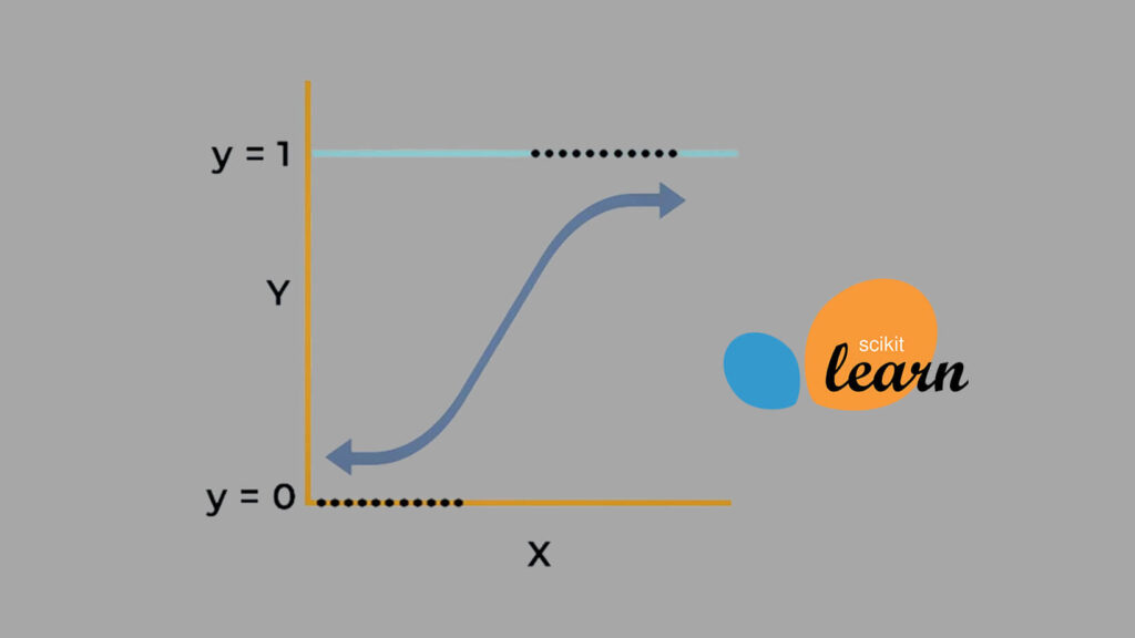
6.1 Sigmoid Function
Logistic regression uses the sigmoid function to convert linear output into a probability between 0 and 1.
\(\sigma(z)=\frac{1}{1+e^{-z}}\)
def sigmoid(z):
    """
    Applies the sigmoid activation function to map input values
    into a range between 0 and 1.

    This function is commonly used in binary classification problems
    (like logistic regression) to convert raw model outputs (logits)
    into interpretable probabilities.

    Mathematically:
        sigmoid(z) = 1 / (1 + e^(-z))

    Parameters:
    -----------
    z : float or np.ndarray
        A scalar or NumPy array of real values (the linear output of a model).

    Returns:
    --------
    float or np.ndarray
        The sigmoid-transformed value(s), ranging from 0 to 1.
    """

    # Prevent extreme values of z from causing numerical overflow in exp()
    # Clipping helps maintain numerical stability for very large or small z
    z = np.clip(z, -500, 500)

    # Compute the sigmoid: 1 / (1 + e^(-z))
return 1 / (1 + np.exp(-z))6.2 Binary Cross-Entropy Loss
We use binary cross-entropy to measure how far off the model’s predictions are:
\(J(w,b)=-\frac{1}{m}\sum_{i=1}^{m}[ylog(\hat{y})+(1-y)log(1-\hat{y})]+\text{regularization}\)
def compute_cost(X, y, w, b, lambda_):
    """
    Computes the regularized binary cross-entropy loss (cost)
    for logistic regression.

    This function measures how well the model's predicted probabilities
    match the actual labels, and includes an L2 regularization term
    to help reduce overfitting.

    Parameters:
    -----------
    X : np.ndarray, shape (m, n)
        Feature matrix where m is the number of examples and
        n is the number of features.

    y : np.ndarray, shape (m,)
        Actual binary labels (0 for ham, 1 for spam).

    w : np.ndarray, shape (n,)
        Weight vector (model parameters for each feature).

    b : float
        Bias term (intercept).

    lambda_ : float
        Regularization strength. Higher values penalize large weights.

    Returns:
    --------
    float
        The total cost: binary cross-entropy + L2 regularization.
    """

    # Number of training examples
    m = X.shape[0]

    # Compute the model output (z = X.w + b)
    z = np.dot(X, w) + b

    # Apply the sigmoid function to get predicted probabilities
    y_hat = sigmoid(z)

    # Clip predicted values to avoid log(0) errors during cost calculation
    y_hat = np.clip(y_hat, 1e-15, 1 - 1e-15)

    # Compute binary cross-entropy loss
    cost = -(1 / m) * np.sum(y * np.log(y_hat) + (1 - y) * np.log(1 - y_hat))

    # Compute L2 regularization term (excluding the bias b)
    reg = (lambda_ / (2 * m)) * np.sum(w ** 2)

    # Total cost = loss + regularization
    return cost + reg
6.3 Training with Gradient Descent
We update the model’s weights w and bias b using the gradients of the loss.
def train_logistic_regression(X, y, learning_rate=0.01, iterations=10000, lambda_=10.0):
    """
    Trains a logistic regression model using batch gradient descent
    and L2 regularization (also known as Ridge regularization).

    Parameters:
    -----------
    X : np.ndarray, shape (m, n)
        Feature matrix where m is the number of examples and
        n is the number of features (e.g., BoW word counts).

    y : np.ndarray, shape (m,)
        Binary labels (0 = ham, 1 = spam).

    learning_rate : float, optional (default=0.01)
        Step size for updating weights during training.

    iterations : int, optional (default=10000)
        Maximum number of training iterations.

    lambda_ : float, optional (default=10.0)
        Regularization strength to reduce overfitting by
        penalizing large weight values (L2 regularization).

    Returns:
    --------
    w : np.ndarray, shape (n,)
        Final optimized weights after training.

    b : float
        Final optimized bias (intercept).

    costs : list of float
        Cost at each iteration — useful for plotting convergence.
    """

    m, n = X.shape  # m = number of samples, n = number of features

    # Initialize weights and bias to zero
    w = np.zeros(n)
    b = 0

    # Keep track of cost at each iteration for visualization
    costs = []

    # Begin gradient descent loop
    for i in range(iterations):
        # Compute model output (z = X.w + b)
        z = np.dot(X, w) + b

        # Apply sigmoid to get predicted probabilities (0 to 1)
        y_hat = sigmoid(z)

        # Compute gradients with respect to weights and bias
        # Includes L2 regularization: (lambda_ / m) * w
        dw = (1 / m) * np.dot(X.T, (y_hat - y)) + (lambda_ / m) * w
        db = (1 / m) * np.sum(y_hat - y)

        # Update parameters using gradient descent
        w -= learning_rate * dw
        b -= learning_rate * db

        # Compute current cost (loss + regularization)
        cost = compute_cost(X, y, w, b, lambda_)
        costs.append(cost)

        if i % 500 == 0 or i == iterations - 1:
            print(f"Iteration {i}: Cost = {cost:.4f}")

        # Converging condition
        if i > 1 and abs(costs[-1] - costs[-2]) < 1e-06:
            print(f"Converged at iteration {i}")
            break

    # Return the learned weights, bias, and the list of costs
return w, b, costsKey Concepts:
- Gradient Descent: Optimizes weights and bias by iteratively reducing the cost function.
- Regularization: Helps prevent overfitting by penalizing large weights.
- Cost Tracking: Allows you to visualize and understand learning progress over time.
- Early Stopping: Stops training if the improvement in cost is negligible.
Step 7: Model Training and Evaluation
Let’s train the model and check how well it performs:
# Train on X_train, y_train
w, b, costs = train_logistic_regression(X_train, y_train, learning_rate=0.01, iterations=10000, lambda_=10.0)Iteration 0: Cost = 0.6667
Iteration 500: Cost = 0.2518
Iteration 1000: Cost = 0.2005
Iteration 1500: Cost = 0.1781
Iteration 2000: Cost = 0.1663
Iteration 2500: Cost = 0.1597
Iteration 3000: Cost = 0.1561
Iteration 3500: Cost = 0.1544
Converged at iteration: 3704
- We can see the model is learning well, as the cost is reducing until it converges at iteration 3704
Visualizing Loss Over Time
plt.plot(costs)
plt.title("Cost Over Iterations")
plt.xlabel("Iteration")
plt.ylabel("Cost")
plt.grid(True)
plt.show()Let’s see how the graph looks like:

You’ll see the cost decrease steadily, a sign that the model is learning.
Step 8: Making Predictions
We classify new emails using our learned weights and bias.
def predict(X, w, b):
    """
    Predicts binary labels (0 or 1) for input feature vectors
    using a trained logistic regression model.

    This function performs the following steps:
    1. Computes the linear combination of inputs and weights (z = X·w + b)
    2. Applies the sigmoid function to convert z into probabilities
    3. Converts probabilities into final class labels:
       - If probability ≥ 0.5, predict 1 (spam)
       - If probability < 0.5, predict 0 (ham)

    Parameters:
    -----------
    X : np.ndarray, shape (m, n)
        Feature matrix of input samples (e.g., Bag-of-Words vectors).

    w : np.ndarray, shape (n,)
        Trained weight vector from the logistic regression model.

    b : float
        Trained bias (intercept) from the model.

    Returns:
    --------
    np.ndarray, shape (m,)
        Predicted class labels (0 or 1) for each input example.
    """

    # Step 1: Compute the raw score (z = X·w + b)
    z = np.dot(X, w) + b

    # Step 2: Apply sigmoid to get probabilities between 0 and 1
    y_hat = sigmoid(z)

    # Step 3: Classify as 1 if probability ≥ 0.5, else 0
return np.where(y_hat > 0.5, 1, 0)Step 9: Evaluating Performance
Let’s measure accuracy:
def accuracy(y_pred, y_true):
    """
    Calculates the classification accuracy of the model.

    Accuracy is the proportion of correct predictions out of
    all predictions made. It's a basic but useful metric for
    evaluating classification performance.

    Parameters:
    -----------
    y_pred : np.ndarray, shape (m,)
        Predicted labels (0 or 1) from the model.

    y_true : np.ndarray, shape (m,)
        Actual true labels (0 or 1) from the dataset.

    Returns:
    --------
    float
        Accuracy score between 0 and 1.
        Multiply by 100 for percentage.
    """
return np.mean(y_pred == y_true)Example Usage
# Evaluate the model on the test set
# y_pred_test: model's predictions
# y_test: actual labels

acc = accuracy(y_pred_test, y_test)

# Print accuracy as a percentage with 2 decimal places
print(f"Test Accuracy: {acc * 100:.2f}%")What This Does:
y_pred == y_truecreates a Boolean array:[True, False, True, …]np.mean(…)treats True as1and False as0, giving the proportion of correct predictions.- Multiplying by 100 gives the percentage (e.g., 0.93 → 93.00%).
This is a strong result, especially given we used raw NumPy and a simple bag-of-words model!
Final Thoughts
In this project, we built a spam classifier from the ground up. Here’s what we did:
- Cleaned and tokenized raw text data.
- Turned emails into numeric features using Bag-of-Words.
- Implemented logistic regression manually.
- Trained with gradient descent and visualized the learning process.
- Evaluated performance with test accuracy.
Key Learnings:
- Machine learning isn’t just calling
.fit(), it’s understanding every component. - Text data is messy, cleaning matters.
- Regularization improves generalization.
- Logistic regression is a great first model for classification.
Want to See the Full Code?
Check out the GitHub repository here: GitHub Repository Link