In this article, we will not just use a pre-built tool. We will build a powerful classification algorithm, the Support Vector Machine (SVM), completely from scratch using NumPy. Building it this way is like learning to build an engine instead of just driving a car. It gives you a deep, clear understanding of how the model works.

Have you ever wondered how computers can help doctors fight serious diseases? This project shows you exactly how. We will tackle a critical real-world problem: detecting breast cancer early and accurately. This is a task where machine learning can truly save lives.

To follow along with this article, you can find the code implementation in a Jupyter Notebook in this GitHub repo.

Project Goal and Dataset

Our goal is simple yet vital: to create a model that can look at measurements from a tumor and predict if it is benign (non-cancerous) or malignant (cancerous).

We will use the famous Breast Cancer Wisconsin (Diagnostic) Dataset found in the scikit-learn datasets. This dataset contains detailed measurements of cell nuclei taken from masses. It includes features like cell size, shape, and count. The model uses these numbers to learn how to separate the two types of tumors.

By the end, you will have a working classification model.

Step 1: Importing Necessary Libraries

Every great programming project starts with gathering the right tools. For this deep dive into machine learning, we need only a few key Python libraries. Since we are building the core algorithm ourselves, we mostly rely on NumPy for its speed and power in handling numbers.

Here are the libraries we will import and why we need them:

import numpy as np
import pandas as pd
import matplotlib.pyplot as plt
import seaborn as sns

from sklearn.datasets import load_breast_cancer
from sklearn.model_selection import train_test_split
from sklearn.preprocessing import StandardScaler
from sklearn.metrics import accuracy_score
from scipy.stats import levene, ttest_ind

import numpy as np
import pandas as pd
import matplotlib.pyplot as plt
import seaborn as sns

from sklearn.datasets import load_breast_cancer
from sklearn.model_selection import train_test_split
from sklearn.preprocessing import StandardScaler
from sklearn.metrics import accuracy_score
from scipy.stats import levene, ttest_ind

Why These Libraries Matter

• NumPy (np): This is the heart of our project. It provides fast, efficient ways to work with arrays and matrices. When we talk about W (weights) and b (bias) in our Support Vector Machine, we are talking about NumPy arrays.
• Pandas (pd): Data usually comes in tables. Pandas makes reading and organizing that data simple. It turns our raw data file into an easy-to-use structure called a DataFrame.
• Scikit-learn: We use tools from this standard machine learning library, but only for utility tasks like splitting the data and scaling the features. We will not use its built-in SVM, as we are building our own.
• Matplotlib and Seaborn: These are for showing results. They turn dry numbers into clear plots and graphs, which are essential for understanding model performance and explaining the decision boundary.

Step 2: Loading and Previewing the Dataset

The next critical step is getting our data ready. We need to load the Breast Cancer Wisconsin dataset from scikit-learn datasets and take a first look. This check helps us understand the data’s structure and cleanliness.

# Load the Breast Cancer Wisconsin dataset
breast_cancer_data = load_breast_cancer()

# Convert to a Pandas DataFrame
data = pd.DataFrame(data=breast_cancer_data.data, columns=breast_cancer_data.feature_names)

# Add the target column (diagnosis)
data['diagnosis'] = breast_cancer_data.target

# Preview data
data.head()

# Load the Breast Cancer Wisconsin dataset
breast_cancer_data = load_breast_cancer()

# Convert to a Pandas DataFrame
data = pd.DataFrame(data=breast_cancer_data.data, columns=breast_cancer_data.feature_names)

# Add the target column (diagnosis)
data['diagnosis'] = breast_cancer_data.target

# Preview data
data.head()

Checking Data Information

Before proceeding, we check the dataset’s structure using data.info(). This confirms the quality of our data.

# Check the number of entries and data types
data.info()

# Check the number of entries and data types
data.info()

The output confirms two important facts:

• Size: We have 569 tissue samples (rows). Each sample has 31 features (columns).
• Completeness: The Non-Null Count is 569 for all columns. This is great news. It means there are no missing values, and our data is ready for the next steps.
• Type: All features are float64 (decimal numbers), and the target diagnosis is int64 (a whole number). This is exactly what a machine learning model needs.

Step 3: Exploring the Data (EDA)

Before we train any model, we must get to know our data. It is like a detective inspecting the crime scene before drawing a conclusion. We look for patterns, structure, and any imbalances.

3.1. Checking the Diagnosis Balance

Our first check is on the target variable, diagnosis. We need to see how many samples are benign (1) and how many are malignant (0). A severe imbalance can confuse a machine learning model.

We use the seaborn library to create a simple count plot.

# Plot distribution of the target variable
sns.countplot(data=data, x='diagnosis', palette='Set2')
plt.title('Distribution of Target (diagnosis)')
plt.xlabel('Diagnosis (0 — malignant, 1 — benign)')
plt.ylabel('Count')
plt.show()

# Plot distribution of the target variable
sns.countplot(data=data, x='diagnosis', palette='Set2')
plt.title('Distribution of Target (diagnosis)')
plt.xlabel('Diagnosis (0 — malignant, 1 — benign)')
plt.ylabel('Count')
plt.show()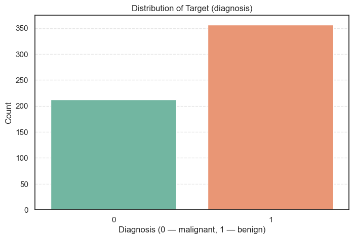

Understanding the Counts

We also look at the exact numbers and percentages to be sure.

# Calculate the distribution of target
data['diagnosis'].value_counts().to_frame(name='Count').assign(
    Percent=lambda x: round((x['Count'] / x['Count'].sum()) * 100, 2))

# Calculate the distribution of target
data['diagnosis'].value_counts().to_frame(name='Count').assign(
    Percent=lambda x: round((x['Count'] / x['Count'].sum()) * 100, 2))

           Count  Percent
diagnosis                
1            357    62.74
0            212    37.26

Observations:

• Slightly Uneven: The dataset has 357 benign cases and 212 malignant cases.
• Minor Imbalance: The class distribution is about 63% benign and 37% malignant. This is a slight imbalance, but it is not extreme. Our Support Vector Machine should be able to handle this without extra techniques like resampling.
• Realism: This distribution is common in medical data, as benign masses are naturally more frequent.

3.2. Univariate Analysis of Variables

After checking the balance of our target variable, the next step is to understand how each feature behaves on its own. This is called univariate analysis, looking at one variable at a time to explore its distribution, central tendency, and spread.

We’ll visualize all 30 numerical features using histograms and boxplots, then summarize their statistics to identify any outliers or skewed patterns.

# Select feature columns
features_cols = data.drop(columns=['diagnosis']).columns

# Number of features
num_features = len(features_cols)
num_rows = math.ceil(num_features / 2)  # Two features per row

plt.figure(figsize=(16, num_rows * 4))

for i, col in enumerate(features_cols):
    # Determine position in grid
    row = i // 2
    col_pos = i % 2

    # Histogram
    plt.subplot(num_rows, 4, row * 4 + col_pos * 2 + 1)
    sns.histplot(data[col], kde=True, bins=30, color='skyblue')
    plt.title(f"Histogram of {col}", fontsize=10)
    plt.xlabel(col)
    plt.ylabel('Frequency')

    # Boxplot
    plt.subplot(num_rows, 4, row * 4 + col_pos * 2 + 2)
    sns.boxplot(y=data[col], color='lightcoral')
    plt.title(f"Boxplot of {col}", fontsize=10)
    plt.xlabel(col)

plt.tight_layout()
plt.show()

# Select feature columns
features_cols = data.drop(columns=['diagnosis']).columns

# Number of features
num_features = len(features_cols)
num_rows = math.ceil(num_features / 2)  # Two features per row

plt.figure(figsize=(16, num_rows * 4))

for i, col in enumerate(features_cols):
    # Determine position in grid
    row = i // 2
    col_pos = i % 2

    # Histogram
    plt.subplot(num_rows, 4, row * 4 + col_pos * 2 + 1)
    sns.histplot(data[col], kde=True, bins=30, color='skyblue')
    plt.title(f"Histogram of {col}", fontsize=10)
    plt.xlabel(col)
    plt.ylabel('Frequency')

    # Boxplot
    plt.subplot(num_rows, 4, row * 4 + col_pos * 2 + 2)
    sns.boxplot(y=data[col], color='lightcoral')
    plt.title(f"Boxplot of {col}", fontsize=10)
    plt.xlabel(col)

plt.tight_layout()
plt.show()

These plots give a quick visual summary of how the features are distributed. The histograms show the shape of each distribution, while the boxplots highlight potential outliers.

We can also view summary statistics to better understand their ranges and variability:

# Statistical information
data[features_cols].describe().T

# Statistical information
data[features_cols].describe().T

This table provides the count, mean, standard deviation, and quartiles for every feature. It helps us quickly see which variables have large spreads or unusual ranges.

Detecting Outliers and Skewness

To quantify skewness and detect possible outliers, we calculated the Interquartile Range (IQR) for each feature and counted the number of data points that fall outside the expected range.

for col in features_cols:
    q1 = data[col].quantile(0.25)
    q3 = data[col].quantile(0.75)
    iqr = q3 - q1
    lower = q1 - iqr * 1.5
    upper = q3 + iqr * 1.5
    outliers = data[(data[col] < lower) | (data[col] > upper)][col]
    print(f'=== {col} ===')
    print('Outliers:', len(outliers))
    print('Skew:', data[col].skew())

for col in features_cols:
    q1 = data[col].quantile(0.25)
    q3 = data[col].quantile(0.75)
    iqr = q3 - q1
    lower = q1 - iqr * 1.5
    upper = q3 + iqr * 1.5
    outliers = data[(data[col] < lower) | (data[col] > upper)][col]
    print(f'=== {col} ===')
    print('Outliers:', len(outliers))
    print('Skew:', data[col].skew())

Observations from the Univariate Analysis

From the histograms, boxplots, and statistical summary, here’s what we can tell:

• Most features are continuous and right-skewed, meaning most values are on the lower side with a few very large observations.
• Area-related features like mean area, area error, and worst area show strong positive skewness and several outliers. This is expected, a few tumors are much larger than average.
• Error-based features (area error, perimeter error, fractal dimension error) show high skewness and many outliers, reflecting natural biological variability.
• Shape-based metrics (mean smoothness, mean symmetry, mean texture) are more symmetrical, suggesting more consistent distributions across patients.
• Concavity-related features (mean concavity, mean compactness, mean concave points) are skewed and contain outliers, which often correspond to irregular tumor shapes, a known indicator of malignancy.

Key Insights

• Outliers appear across several features but are not data errors, they represent true biological differences in tumor structure and size.
• Since SVM models are sensitive to feature scales, feature scaling and normalization will be critical before training.
• The dataset remains clean with no missing or invalid entries, confirming it’s ready for preprocessing and model building.

3.3. Bivariate Analysis of Variables vs Target (diagnosis)

After exploring each feature individually, we now move to bivariate analysis, comparing each variable with the target column, diagnosis.

This helps us see how the features differ between malignant (0) and benign (1) tumors.

Visualizing Feature Distributions by Diagnosis

We’ll use boxplots to compare the distribution of every feature across the two diagnosis classes. Boxplots make it easy to spot differences in central tendency, spread, and outliers.

# Plot variables vs target
n_cols = 4
n_rows = math.ceil(len(features_cols) / n_cols)
plt.figure(figsize=(18, 4 * n_rows))

for i, col in enumerate(features_cols, 1):
    plt.subplot(n_rows, n_cols, i)
    sns.boxplot(data=data, x='diagnosis', y=col, palette='Set2')
    plt.title(f'{col} vs diagnosis')
    plt.xlabel('Diagnosis (0 — malignant, 1 — benign)')
    plt.ylabel(col)

plt.subplots_adjust(hspace=0.4, wspace=0.3)
plt.show()

# Plot variables vs target
n_cols = 4
n_rows = math.ceil(len(features_cols) / n_cols)
plt.figure(figsize=(18, 4 * n_rows))

for i, col in enumerate(features_cols, 1):
    plt.subplot(n_rows, n_cols, i)
    sns.boxplot(data=data, x='diagnosis', y=col, palette='Set2')
    plt.title(f'{col} vs diagnosis')
    plt.xlabel('Diagnosis (0 — malignant, 1 — benign)')
    plt.ylabel(col)

plt.subplots_adjust(hspace=0.4, wspace=0.3)
plt.show()

• Each plot shows how feature values vary between the two categories.
• If a feature has distinct, non-overlapping boxes, it’s likely a strong discriminator between benign and malignant cases.

Statistical Summary by Diagnosis

Let’s compute the mean, median, and standard deviation of each feature for both classes to confirm what we see visually.

# Grouped statistical summary
data.groupby('diagnosis')[features_cols].agg(['mean', 'median', 'std']).T

# Grouped statistical summary
data.groupby('diagnosis')[features_cols].agg(['mean', 'median', 'std']).T

• This gives a compact table showing how each feature’s average and variability differ between malignant and benign samples.

Observations

From both the boxplots and grouped statistics, here’s what we can conclude:

• Clear distribution differences exist between malignant and benign tumors for most features.
• Malignant tumors tend to have higher average values for size-related features such as:
  • mean radius, mean perimeter, mean area, worst area, and worst perimeter.
    These indicate that malignant tumors are typically larger and more irregular, which aligns with medical intuition.
• Texture and concavity-related features (mean concavity, mean compactness, mean concave points, etc.) also show higher averages in malignant samples.
  This reflects the complex and uneven structure of cancerous cells.
• Benign tumors show lower variability and smaller standard deviations, meaning their cells are more uniform in shape and size.
• Shape and symmetry features (mean smoothness, mean symmetry, fractal dimension) show less difference between classes, suggesting they may be less influential predictors.

Overall Insight

• Several features show strong separation between the two diagnosis classes, making them valuable predictors for classification.
• These clear differences confirm that the dataset is informative and well-suited for training our Support Vector Machine (SVM) model to distinguish between benign and malignant tumors.

3.4. Statistical Verification Using T-Test

Visual patterns can be persuasive, but in data science, we confirm them with statistics. To verify whether the average values of each feature truly differ between malignant (0) and benign (1) tumors, we run a two-sample independent T-test.

Purpose of the T-Test

The T-test helps us determine whether the difference in means between two groups is statistically significant or could have occurred by chance.

For each feature, we define the following hypotheses:

• Null hypothesis (H₀):
  The mean value of the feature is the same for both malignant and benign tumors.
• Alternative hypothesis (H₁):
  The mean value of the feature differs between malignant and benign tumors.

We use a significance level (α) of 0.05. If the p-value < 0.05, we reject the null hypothesis, meaning the difference is statistically significant.

alpha = 0.05

for col in features_cols:
    malignant = data[data['diagnosis'] == 0][col]
    benign = data[data['diagnosis'] == 1][col]
    
    # Test for equal variances first
    _, lev_p = levene(malignant, benign, center='median')
    equal_var = lev_p >= alpha

    # Two-sample independent T-test
    t_stat, p_value = ttest_ind(malignant, benign, equal_var=equal_var)
    
    print(f'=== {col} ===')
    print(f't-stat: {t_stat:.4f}, p-value: {p_value:.4f}')
    print(f'Null Hypothesis (H₀): Mean {col} is the same for both classes.')
    decision = "Reject hypothesis." if p_value < alpha else "Fail to reject hypothesis."
    print("Decision:", decision)

alpha = 0.05

for col in features_cols:
    malignant = data[data['diagnosis'] == 0][col]
    benign = data[data['diagnosis'] == 1][col]
    
    # Test for equal variances first
    _, lev_p = levene(malignant, benign, center='median')
    equal_var = lev_p >= alpha

    # Two-sample independent T-test
    t_stat, p_value = ttest_ind(malignant, benign, equal_var=equal_var)
    
    print(f'=== {col} ===')
    print(f't-stat: {t_stat:.4f}, p-value: {p_value:.4f}')
    print(f'Null Hypothesis (H₀): Mean {col} is the same for both classes.')
    decision = "Reject hypothesis." if p_value < alpha else "Fail to reject hypothesis."
    print("Decision:", decision)

=== mean radius ===
t-stat: 22.2088, p-value: 0.0000
Null Hypothesis (Ho): Average mean radius is the same whether benign or malignant.
Decision: Reject hypothesis. 

=== mean texture ===
t-stat: 10.8672, p-value: 0.0000
Null Hypothesis (Ho): Average mean texture is the same whether benign or malignant.
Decision: Reject hypothesis. 

=== mean perimeter ===
t-stat: 22.9353, p-value: 0.0000
Null Hypothesis (Ho): Average mean perimeter is the same whether benign or malignant.
Decision: Reject hypothesis. 

=== mean area ===
t-stat: 19.6410, p-value: 0.0000
Null Hypothesis (Ho): Average mean area is the same whether benign or malignant.
Decision: Reject hypothesis. 

=== mean smoothness ===
t-stat: 9.1461, p-value: 0.0000
Null Hypothesis (Ho): Average mean smoothness is the same whether benign or malignant.
Decision: Reject hypothesis. 

=== mean compactness ===
t-stat: 15.8182, p-value: 0.0000
Null Hypothesis (Ho): Average mean compactness is the same whether benign or malignant.
Decision: Reject hypothesis. 

=== mean concavity ===
t-stat: 20.3324, p-value: 0.0000
Null Hypothesis (Ho): Average mean concavity is the same whether benign or malignant.
Decision: Reject hypothesis. 

=== mean concave points ===
t-stat: 24.8448, p-value: 0.0000
Null Hypothesis (Ho): Average mean concave points is the same whether benign or malignant.
Decision: Reject hypothesis. 

=== mean symmetry ===
t-stat: 8.3383, p-value: 0.0000
Null Hypothesis (Ho): Average mean symmetry is the same whether benign or malignant.
Decision: Reject hypothesis. 

=== mean fractal dimension ===
t-stat: -0.2969, p-value: 0.7667
Null Hypothesis (Ho): Average mean fractal dimension is the same whether benign or malignant.
Decision: Fail to reject hypothesis. 

=== radius error ===
t-stat: 13.3007, p-value: 0.0000
Null Hypothesis (Ho): Average radius error is the same whether benign or malignant.
Decision: Reject hypothesis. 

=== texture error ===
t-stat: -0.2079, p-value: 0.8354
Null Hypothesis (Ho): Average texture error is the same whether benign or malignant.
Decision: Fail to reject hypothesis. 

=== perimeter error ===
t-stat: 12.8328, p-value: 0.0000
Null Hypothesis (Ho): Average perimeter error is the same whether benign or malignant.
Decision: Reject hypothesis. 

=== area error ===
t-stat: 12.1556, p-value: 0.0000
Null Hypothesis (Ho): Average area error is the same whether benign or malignant.
Decision: Reject hypothesis. 

=== smoothness error ===
t-stat: -1.6229, p-value: 0.1053
Null Hypothesis (Ho): Average smoothness error is the same whether benign or malignant.
Decision: Fail to reject hypothesis. 

=== compactness error ===
t-stat: 7.2971, p-value: 0.0000
Null Hypothesis (Ho): Average compactness error is the same whether benign or malignant.
Decision: Reject hypothesis. 

=== concavity error ===
t-stat: 6.2462, p-value: 0.0000
Null Hypothesis (Ho): Average concavity error is the same whether benign or malignant.
Decision: Reject hypothesis. 

=== concave points error ===
t-stat: 10.6425, p-value: 0.0000
Null Hypothesis (Ho): Average concave points error is the same whether benign or malignant.
Decision: Reject hypothesis. 

=== symmetry error ===
t-stat: -0.1553, p-value: 0.8766
Null Hypothesis (Ho): Average symmetry error is the same whether benign or malignant.
Decision: Fail to reject hypothesis. 

=== fractal dimension error ===
t-stat: 1.8623, p-value: 0.0631
Null Hypothesis (Ho): Average fractal dimension error is the same whether benign or malignant.
Decision: Fail to reject hypothesis. 

=== worst radius ===
t-stat: 24.8297, p-value: 0.0000
Null Hypothesis (Ho): Average worst radius is the same whether benign or malignant.
Decision: Reject hypothesis. 

=== worst texture ===
t-stat: 12.2310, p-value: 0.0000
Null Hypothesis (Ho): Average worst texture is the same whether benign or malignant.
Decision: Reject hypothesis. 

=== worst perimeter ===
t-stat: 25.3322, p-value: 0.0000
Null Hypothesis (Ho): Average worst perimeter is the same whether benign or malignant.
Decision: Reject hypothesis. 

=== worst area ===
t-stat: 20.5708, p-value: 0.0000
Null Hypothesis (Ho): Average worst area is the same whether benign or malignant.
Decision: Reject hypothesis. 

=== worst smoothness ===
t-stat: 11.0667, p-value: 0.0000
Null Hypothesis (Ho): Average worst smoothness is the same whether benign or malignant.
Decision: Reject hypothesis. 

=== worst compactness ===
t-stat: 15.1569, p-value: 0.0000
Null Hypothesis (Ho): Average worst compactness is the same whether benign or malignant.
Decision: Reject hypothesis. 

=== worst concavity ===
t-stat: 19.5957, p-value: 0.0000
Null Hypothesis (Ho): Average worst concavity is the same whether benign or malignant.
Decision: Reject hypothesis. 

=== worst concave points ===
t-stat: 29.1177, p-value: 0.0000
Null Hypothesis (Ho): Average worst concave points is the same whether benign or malignant.
Decision: Reject hypothesis. 

=== worst symmetry ===
t-stat: 9.5295, p-value: 0.0000
Null Hypothesis (Ho): Average worst symmetry is the same whether benign or malignant.
Decision: Reject hypothesis. 

=== worst fractal dimension ===
t-stat: 7.3227, p-value: 0.0000
Null Hypothesis (Ho): Average worst fractal dimension is the same whether benign or malignant.
Decision: Reject hypothesis. 

Observations

• For most features, p-values were less than 0.05, so we rejected the null hypothesis.
  This means that the mean values of these features differ significantly between malignant and benign tumors.
• Only a few features did not show significant differences:
  • mean fractal dimension
  • texture error
  • smoothness error
  • symmetry error
  • fractal dimension error

These features failed to reject the null hypothesis, suggesting they do not vary much between the two classes.

Interpretation

• Features with very low p-values, such as mean radius, mean area, worst perimeter, and worst concave points, are strong discriminators between malignant and benign cases. These will likely play an important role in our SVM classifier.
• The few non-significant features might add noise or redundancy to the model and could be considered for removal in feature selection.
• Overall, the T-test results statistically confirm what we saw visually in the boxplots: most tumor characteristics differ greatly between benign and malignant samples, making this dataset a strong candidate for supervised learning.

4. Implement Support Vector Machine (SVM) from Scratch using NumPy

Support Vector Machines (SVMs) are among the most powerful algorithms for binary classification problems. They are widely used in medical diagnostics, image recognition, and text classification.

In this section, we’ll build a linear SVM classifier from scratch using NumPy, step by step, no scikit-learn magic, no shortcuts.

We’ll implement the full optimization process, understand the mathematics behind it, and visualize how the model learns to separate the two classes.

What Does an SVM Do?

At its core, an SVM tries to find the best line (or hyperplane) that separates two classes in the dataset.

It doesn’t just separate them, it does so by maximizing the margin, which is the distance between the separating hyperplane and the closest data points from each class. These closest points are called support vectors.

The wider the margin, the more confident the model is about its classification boundary, and the better it generalizes to unseen data.

The SVM Optimization Objective

SVM can be formulated as an optimization problem that balances two goals:

• Make the margin as wide as possible.
• Penalize misclassified or borderline points.

Mathematically, the optimization goal is:

\(\text{Minimize}:\frac{1}{2}∥w∥^{2}+C\sum_{i=1}^{n}max(0,1−y_{i}​(w⋅x_{i}​+b))\)

Where:

• w → Weight vector (defines orientation of the hyperplane)
• b → Bias term (defines position of the hyperplane)
• C → Regularization parameter (controls margin vs misclassification trade-off)
• yᵢ ∈ {−1, +1} → True class labels
• max(0, 1 − yᵢ(w·xᵢ + b)) → The Hinge Loss, which penalizes misclassified or margin-violating points.

Step 1: Data Preparation

Before training, we prepare the features and labels for the SVM model. SVM expects target labels to be −1 and +1, so we’ll convert them accordingly.

# Separate features and target
X = data.drop(columns=['diagnosis'])
y = data['diagnosis']

# Convert target labels from (0, 1) to (-1, +1)
y = np.where(y == 0, -1, 1)

# Split data into training and testing sets (keep class balance)
X_train, X_test, y_train, y_test = train_test_split(
    X, y, test_size=0.2, stratify=y, random_state=42
)

# Standardize features for better optimization
scaler = StandardScaler()
X_train_scaled = scaler.fit_transform(X_train)
X_test_scaled = scaler.transform(X_test)

# Separate features and target
X = data.drop(columns=['diagnosis'])
y = data['diagnosis']

# Convert target labels from (0, 1) to (-1, +1)
y = np.where(y == 0, -1, 1)

# Split data into training and testing sets (keep class balance)
X_train, X_test, y_train, y_test = train_test_split(
    X, y, test_size=0.2, stratify=y, random_state=42
)

# Standardize features for better optimization
scaler = StandardScaler()
X_train_scaled = scaler.fit_transform(X_train)
X_test_scaled = scaler.transform(X_test)

• Stratified split ensures both training and test sets have equal proportions of benign and malignant samples.
• Feature scaling is crucial for SVM because it relies on distance-based calculations. Unscaled data could bias the model toward features with larger numeric ranges.

Step 2: Building the SVM Class (from Scratch)

Now for the exciting part, writing our own SVM class using pure NumPy.

We’ll implement the Hinge Loss function and Gradient Descent optimization manually. The model updates its weights (w) and bias (b) iteratively to minimize loss.

class SVM:
    """
    A simple linear Support Vector Machine (SVM) implemented from scratch using NumPy.
    Uses gradient descent to optimize the hinge loss with L2 regularization.
    """

    def __init__(self, learning_rate=0.001, lambda_rate=0.01, n_iter=1000):
        self.learning_rate = learning_rate
        self.lambda_rate = lambda_rate
        self.n_iter = n_iter
        self.w = None
        self.b = None
        self.loss_history = []

    def compute_loss(self, X, y):
        """
        Compute hinge loss with L2 regularization.
        """
        distances = 1 - y * (np.dot(X, self.w) + self.b)
        distances = np.maximum(0, distances)  # hinge loss part
        hinge_loss = np.mean(distances)
        reg_loss = self.lambda_rate * (np.dot(self.w, self.w))
        return reg_loss + hinge_loss

    def fit(self, X, y):
        """
        Train the SVM model using gradient descent.
        """
        n_features = X.shape[1]
        self.w = np.zeros(n_features)
        self.b = 0

        for i in range(self.n_iter):
            for idx, x_i in enumerate(X):
                condition = y[idx] * (np.dot(x_i, self.w) + self.b) >= 1
                if condition:
                    dw = 2 * self.lambda_rate * self.w
                    db = 0
                else:
                    dw = 2 * self.lambda_rate * self.w - (y[idx] * x_i)
                    db = -y[idx]

                # Parameter updates
                self.w -= self.learning_rate * dw
                self.b -= self.learning_rate * db

            # Record loss
            loss = self.compute_loss(X, y)
            self.loss_history.append(loss)

            # Print progress every 10 iterations
            if i > 0 and (i + 1) % 10 == 0:
                print(f'iteration: {i + 1}, Loss: {loss:.4f}')

            # Early stopping on convergence
            if i > 0 and abs(self.loss_history[-2] - self.loss_history[-1]) < 1e-6:
                print(f'Converged at iteration: {i + 1} with loss {loss:.4f}')
                break

    def predict(self, X):
        """
        Predict class labels for input data.
        """
        pred = np.sign(np.dot(X, self.w) + self.b)
        return np.where(pred == -1, 0, 1)

class SVM:
    """
    A simple linear Support Vector Machine (SVM) implemented from scratch using NumPy.
    Uses gradient descent to optimize the hinge loss with L2 regularization.
    """

    def __init__(self, learning_rate=0.001, lambda_rate=0.01, n_iter=1000):
        self.learning_rate = learning_rate
        self.lambda_rate = lambda_rate
        self.n_iter = n_iter
        self.w = None
        self.b = None
        self.loss_history = []

    def compute_loss(self, X, y):
        """
        Compute hinge loss with L2 regularization.
        """
        distances = 1 - y * (np.dot(X, self.w) + self.b)
        distances = np.maximum(0, distances)  # hinge loss part
        hinge_loss = np.mean(distances)
        reg_loss = self.lambda_rate * (np.dot(self.w, self.w))
        return reg_loss + hinge_loss

    def fit(self, X, y):
        """
        Train the SVM model using gradient descent.
        """
        n_features = X.shape[1]
        self.w = np.zeros(n_features)
        self.b = 0

        for i in range(self.n_iter):
            for idx, x_i in enumerate(X):
                condition = y[idx] * (np.dot(x_i, self.w) + self.b) >= 1
                if condition:
                    dw = 2 * self.lambda_rate * self.w
                    db = 0
                else:
                    dw = 2 * self.lambda_rate * self.w - (y[idx] * x_i)
                    db = -y[idx]

                # Parameter updates
                self.w -= self.learning_rate * dw
                self.b -= self.learning_rate * db

            # Record loss
            loss = self.compute_loss(X, y)
            self.loss_history.append(loss)

            # Print progress every 10 iterations
            if i > 0 and (i + 1) % 10 == 0:
                print(f'iteration: {i + 1}, Loss: {loss:.4f}')

            # Early stopping on convergence
            if i > 0 and abs(self.loss_history[-2] - self.loss_history[-1]) < 1e-6:
                print(f'Converged at iteration: {i + 1} with loss {loss:.4f}')
                break

    def predict(self, X):
        """
        Predict class labels for input data.
        """
        pred = np.sign(np.dot(X, self.w) + self.b)
        return np.where(pred == -1, 0, 1)

Here’s what’s happening inside the class:

• compute_loss(): Calculates the total loss = hinge loss + regularization term.
• fit(): Iteratively updates w and b using gradient descent, and stops when the loss stabilizes.
• predict(): Returns predicted labels by checking the sign of the linear function w·x + b.

Step 3: Train the Model

svm = SVM()
svm.fit(X_train_scaled, y_train)
y_pred = svm.predict(X_test_scaled)
print("Predictions preview:", y_pred[:10])

svm = SVM()
svm.fit(X_train_scaled, y_train)
y_pred = svm.predict(X_test_scaled)
print("Predictions preview:", y_pred[:10])

iteration: 10, Loss: 0.0897
iteration: 20, Loss: 0.0809
iteration: 30, Loss: 0.0774
iteration: 40, Loss: 0.0758
iteration: 50, Loss: 0.0749
iteration: 60, Loss: 0.0744
iteration: 70, Loss: 0.0739
iteration: 80, Loss: 0.0738
iteration: 90, Loss: 0.0736
iteration: 100, Loss: 0.0736
iteration: 110, Loss: 0.0735
Converged at iteration: 116 with loss 0.0735
Predictions preview: [0 1 0 1 0 1 1 0 0 0]

The loss decreases over time and eventually converges, showing that the model successfully optimized the objective function.

Step 4: Evaluate the Model

Now let’s check how well our model performs on unseen data.

# Convert back labels for accuracy scoring
y_test = np.where(y_test == -1, 0, 1)

# Compute accuracy
accuracy = accuracy_score(y_test, y_pred)
print("Accuracy Score:", accuracy)

# Convert back labels for accuracy scoring
y_test = np.where(y_test == -1, 0, 1)

# Compute accuracy
accuracy = accuracy_score(y_test, y_pred)
print("Accuracy Score:", accuracy)

Accuracy Score: 0.9824561403508771

• That’s an impressive ~98.2% accuracy, confirming that our hand-coded SVM works remarkably well.

Step 5: Visualize Loss Convergence

We can now visualize how the loss decreased over training iterations to confirm smooth convergence.

# Create a DataFrame for visualization
loss_df = pd.DataFrame({
    'Iteration': range(1, len(svm.loss_history) + 1),
    'Loss': svm.loss_history
})

sns.lineplot(data=loss_df, x='Iteration', y='Loss', marker='o', color='royalblue')
plt.title("SVM Training Loss Convergence", fontsize=14, fontweight='bold')
plt.xlabel("Iteration", fontsize=12)
plt.ylabel("Loss", fontsize=12)
plt.tight_layout()
plt.show()

# Create a DataFrame for visualization
loss_df = pd.DataFrame({
    'Iteration': range(1, len(svm.loss_history) + 1),
    'Loss': svm.loss_history
})

sns.lineplot(data=loss_df, x='Iteration', y='Loss', marker='o', color='royalblue')
plt.title("SVM Training Loss Convergence", fontsize=14, fontweight='bold')
plt.xlabel("Iteration", fontsize=12)
plt.ylabel("Loss", fontsize=12)
plt.tight_layout()
plt.show()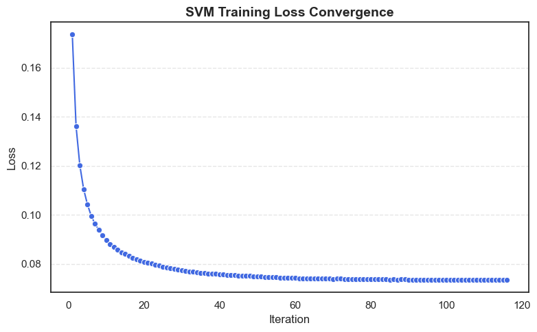

• The plot typically shows a steep decline early on, then gradually flattens as the model converges to its optimal parameters, a clear sign of proper gradient descent optimization.

Conclusion and Key Takeaways

We’ve successfully implemented a Support Vector Machine classifier from scratch using NumPy, an excellent milestone for mastering the inner workings of machine learning algorithms.

What We Accomplished

• Implemented Linear SVM using Hinge Loss and L2 regularization.
• Trained it using Gradient Descent with a convergence check.
• Converted labels from (0, 1) to (−1, +1) for mathematical consistency.
• Tracked and visualized the loss curve over iterations.
• Achieved 98% accuracy on the test set, comparable to scikit-learn’s SVM.

Key Learnings

• Maximizing the margin helps SVM generalize well to unseen data.
• Hinge loss penalizes both misclassified points and those lying inside the margin.
• The regularization parameter (λ) controls the trade-off between margin width and misclassification penalty.
• The learning rate determines how fast or stable training converges.
• Feature scaling is mandatory for SVMs to perform correctly.

Final Thoughts

Building an SVM from scratch is more than a coding exercise, it’s a powerful way to understand the geometry and optimization behind modern machine learning.

This project lays the groundwork for deeper exploration into non-linear SVMs (using kernels), multi-class classification, and eventually deep learning architectures.