A Step-by-Step Beginner’s Guide Using the MNIST Dataset
If you’ve ever taken a machine learning course, you’ve likely come across the MNIST dataset. A collection of 70,000 grayscale images of handwritten digits ranging from 0 to 9. It’s often described as the “Hello, World” of computer vision.
Most tutorials show how to build models for this task using popular deep learning libraries like TensorFlow or PyTorch. These frameworks are powerful, but they abstract away so much of what’s happening under the hood.
In this project, I decided to strip away all the abstraction and build a neural network from scratch, using nothing but NumPy. No Keras. No scikit-learn. No high-level APIs. Just a raw, honest neural network implementation — layer by layer, function by function.
The goal? To truly understand how neural networks work at the fundamental level, it is essential to grasp how images are processed, how neurons activate, how predictions are made, and how the model learns from mistakes.
What is MNIST and Why Use It?
The MNIST dataset contains 70,000 images of handwritten digits:
- 60,000 for training and
- 10,000 for testing.
Each image is 28×28 pixels, in grayscale, and labeled with the correct digit (0–9). That means every image can be flattened into a 784-dimensional vector.
MNIST is simple enough to let us focus on core learning mechanics, but complex enough to make the results meaningful.
To follow along with this guide, you can find the code implementation in a Jupyter notebook in this GitHub repo. Let’s start by loading and visualizing the data.
Step 1: Loading and Exploring the Dataset
We’ll use tensorflow.keras.datasets to load MNIST, just to avoid dealing with downloading and parsing files manually. This is the only exception we make for convenience.
from tensorflow.keras.datasets import mnist

# Load MNIST dataset
(X_train, y_train), (X_test, y_test) = mnist.load_data()This gives us:
X_train: 60,000 images of shape (28, 28)y_train: corresponding labels (integers from 0–9)X_test,y_test: the 10,000 test samples
Let’s visualize a few digits to get a feel for the data:
plt.figure(figsize=(10, 2))
for i in range(10):
    plt.subplot(1, 10, i + 1)
    plt.imshow(X_train[i], cmap="gray")
    plt.title(str(y_train[i]))
    plt.axis("off")
plt.suptitle("Sample MNIST Digits")
plt.show()You should see a row of familiar digits, perhaps a messy 5, a crisp 0, or a loopy 2. These are the raw inputs we’ll teach our neural network to recognize.

Step 2: Preprocessing the Data
Neural networks don’t work well with 2D image matrices or pixel values ranging from 0 to 255. Before feeding images into a neural network, we need to:
- Flatten the 28×28 images into 1D vectors (784 values).
- Normalize pixel values from [0, 255] to [0, 1] for stable training.
- One-hot encode labels (e.g., “3” → [0, 0, 0, 1, 0, 0, 0, 0, 0, 0]).
2.1 Flattening
We reshape each image from 28×28 pixels into a 784-length row vector:
X_train_flat = X_train.reshape(X_train.shape[0], -1)
X_test_flat = X_test.reshape(X_test.shape[0], -1)This gives us a matrix of shape (60000, 784) — one row per image, one column per pixel.
2.2 Normalization
Next, we scale the pixel values to the range [0, 1]. This helps the model learn faster by keeping input values consistent and small.
We will apply min-max normalization to scale pixel values from the range [0, 255] to [0, 1]. Pixels usually go up to 255. So dividing by 255 normalizes pixel intensity values to a standard range of [0, 1], helping the neural network learn more efficiently.
X_train_flat = X_train_flat / 255.0
X_test_flat = X_test_flat / 255.02.3 One-Hot Encoding
The labels 0 through 9 are just integers, but we want the output of the model to be probabilities across 10 classes. So we convert each label into a one-hot vector:
import numpy as np

def one_hot_encode(y, num_classes=10):
    """
    Converts a vector of class labels (e.g., [3, 0, 4]) into one-hot encoded format.

    One-hot encoding transforms each label into a vector of zeros with a 1
    in the position of the class index. For example:
        Label 3 → [0, 0, 0, 1, 0, 0, 0, 0, 0, 0]

    Parameters:
    -----------
    y : array-like, shape (m,)
        A list or array of integer class labels (e.g., digits 0 through 9).

    num_classes : int
        The total number of classes. Default is 10 (for digits 0–9 in MNIST).

    Returns:
    --------
    one_hot : np.ndarray, shape (m, num_classes)
        A 2D array where each row is a one-hot vector representing a label.
    """

    # Create an array of zeros with shape (number of samples, number of classes)
    one_hot = np.zeros((len(y), num_classes))

    # Set the correct class index to 1 for each sample
    # For example, if y = [2, 0, 3], this sets:
    # [0, 0, 1, 0, ...], [1, 0, 0, 0, ...], [0, 0, 0, 1, ...]
    one_hot[np.arange(len(y)), y] = 1

return one_hotNow, for example, label 3 becomes:
[0, 0, 0, 1, 0, 0, 0, 0, 0, 0]
Step 3: Defining the Neural Network Architecture
We’ll use a 2-layer feedforward neural network:
- Input layer: 784 neurons (1 for each pixel)
- Hidden layer: 128 neurons, ReLU activation
- Output layer: 10 neurons (1 for each digit), Softmax activation
Key Components:
- ReLU Activation: Introduces non-linearity (outputs max(0, input)).
- Softmax Activation: Converts outputs into probabilities (sums to 1).
- Weight Initialization: Small random values to break symmetry.
Let’s initialize the weights and biases:
# Set a fixed seed for reproducibility
np.random.seed(0)

# Initialize weights for the first layer (input → hidden).
# Input has 784 features (28x28 pixels), and we choose 128 neurons in the hidden layer.
# We multiply by 0.01 to keep initial weights small, which helps with training stability.
W1 = 0.01 * np.random.randn(784, 128)

# Initialize bias for the hidden layer to zeros (one bias per hidden neuron).
# Shape: (1, 128) to match the number of neurons in the hidden layer.
b1 = np.zeros((1, 128))

# Initialize weights for the second layer (hidden → output).
# The hidden layer has 128 neurons and the output layer has 10 classes (digits 0–9).
W2 = 0.01 * np.random.randn(128, 10)

# Initialize bias for the output layer (one bias per output neuron).
# Shape: (1, 10) to match the 10 output classes.
b2 = np.zeros((1, 10))W1,b1: Weights and biases for the first layer.W2,b2: Weights and biases for the output layer.
We multiply inputs by weights, add bias, apply activations, and pass the results forward.
Step 4: Forward Propagation
4.1 ReLU Activation
ReLU (Rectified Linear Unit) is a simple, effective activation function that replaces all negative values with zero. It is defined as:
\(ReLU(z)=max(0,z)\)
Where:
- Input: A real number
z(typically the output of a linear transformation like \(z=w^{T}x+b\)). - Output:
- If \(z > 0\), returns
z. - If \(z\le 0\), returns
0.
- If \(z > 0\), returns
def relu(z):
    """
    ReLU sets all negative input values to zero and leaves positive
    values unchanged. It is commonly used in hidden layers of neural
    networks to introduce non-linearity and avoid vanishing gradients.

    Parameters:
    -----------
    z : np.ndarray
        The input array (can be scalar, vector, or matrix) representing
        the output of a linear transformation (e.g., z = XW + b).

    Returns:
    --------
    np.ndarray
        An array with the same shape as z, where all negative values
        have been replaced by 0.
    """

    # Replace negative values with 0 and return the result
return np.maximum(0, z)4.2 Softmax Activation
Softmax turns raw scores into probabilities that sum to 1.
For a vector of logits z = [z1, z2, ..., zK] (where K = number of classes), Softmax computes:
\(\text{Softmax}(z_{i})=\frac{e^{z_{i}}}{\sum_{j=1}^{K}e^{z_{j}}}\)
- Input: Raw scores (logits) from the output layer.
- Output: Probability distribution over
Kclasses.
def softmax(z):
    """
    The softmax function converts raw scores (logits) into probabilities
    that sum to 1. It is typically used in the output layer of a
    multiclass classification neural network.

    For each sample:
        softmax(z_i) = exp(z_i) / sum(exp(z_j) for all classes j)

    Parameters:
    -----------
    z : np.ndarray, shape (m, n)
        The input array of raw scores (logits), where:
        - m is the number of samples (batch size)
        - n is the number of classes

    Returns:
    --------
    np.ndarray, shape (m, n)
        The softmax-transformed output where each row is a probability
        distribution over the n classes for each sample.
    """

    # Subtract the max of each row from each value in that row
    # This improves numerical stability and avoids overflow in exp()
    exp_values = np.exp(z - np.max(z, axis=1, keepdims=True))

    # Normalize each row by dividing by the sum of its exponentiated values
return exp_values / np.sum(exp_values, axis=1, keepdims=True)4.3 The Forward Pass
Putting it all together:
def forward_pass(x):
    """
    This function takes input data and processes it through:
    1. A linear transformation (input layer → hidden layer)
    2. ReLU activation in the hidden layer
    3. A second linear transformation (hidden layer → output layer)
    4. Softmax activation in the output layer (for multiclass classification)

    Parameters:
    -----------
    x : np.ndarray, shape (m, 784)
        Input data where:
        - m is the number of examples
        - 784 is the flattened pixel count of a 28x28 image

    Returns:
    --------
    z1 : np.ndarray
        The linear output before activation in the hidden layer.

    a1 : np.ndarray
        The ReLU-activated output of the hidden layer.

    z2 : np.ndarray
        The linear output before activation in the output layer.

    a2 : np.ndarray
        The softmax-activated output probabilities (final predictions).
    """

    # First linear transformation: input to hidden layer
    z1 = np.dot(x, W1) + b1

    # Apply ReLU activation to introduce non-linearity
    a1 = relu(z1)

    # Second linear transformation: hidden to output layer
    z2 = np.dot(a1, W2) + b2

    # Apply softmax activation to produce output probabilities
    a2 = softmax(z2)

    # Return all intermediate values for use in backpropagation
return z1, a1, z2, a2This outputs a vector of 10 probabilities for each digit image, representing the model’s “confidence” in each class.
Step 5: Loss Function – Categorical Cross-Entropy
The loss function tells us how wrong the model is. For multiclass classification, we use categorical cross-entropy:
\(L_{batch}=-\frac{1}{N}\sum_{i=1}^{N}log(\hat{y}^{(i)}_{\text{correct class}})\)
def categorical_cross_entropy(y_true, y_pred):
    """
    This loss function is commonly used for multiclass classification tasks.
    It measures how well the predicted probability distribution (from softmax)
    matches the actual one-hot encoded labels.

    Formula:
        Loss = -1/m * Σ(log(probability of correct class))

    Parameters:
    -----------
    y_true : np.ndarray, shape (m, n)
        One-hot encoded true labels where:
        - m is the number of samples
        - n is the number of classes
        Example: [0, 0, 1, 0, 0, 0, 0, 0, 0, 0] for class 2

    y_pred : np.ndarray, shape (m, n)
        Predicted class probabilities from the softmax output.

    Returns:
    --------
    float
        The average cross-entropy loss across all samples.
    """

    # Prevent numerical instability: clip values to avoid log(0) or log(1)
    y_pred = np.clip(y_pred, 1e-7, 1 - 1e-7)

    # Extract the predicted probability of the correct class for each sample
    # Since y_true is one-hot encoded, only the correct class has a 1
    correct_probs = np.sum(y_true * y_pred, axis=1)

    # Compute the average negative log-likelihood
return -np.mean(np.log(correct_probs))If the model predicts a low probability for the correct class, the loss is high. If it’s confident and correct, the loss is low.
Step 6: Backpropagation and Training
Now comes the learning part. We calculate how the loss changes with respect to each parameter, then adjust the weights and biases in the direction that reduces the loss.
This is backpropagation + gradient descent.
We define a simple training loop:
learning_rate = 0.5
iterations = 2000
losses = []

for i in range(iterations):
    # Forward pass
    Z1, A1, Z2, A2 = forward_pass(X_train_flat)

    # Compute loss
    loss = categorical_cross_entropy(y_train_encoded, A2)
    losses.append(loss)

    # Backpropagation
    dZ2 = A2 - y_train_encoded
    dW2 = np.dot(A1.T, dZ2) / X_train_flat.shape[0]
    db2 = np.sum(dZ2, axis=0, keepdims=True) / X_train_flat.shape[0]

    dA1 = np.dot(dZ2, W2.T)
    dZ1 = dA1 * (Z1 > 0)
    dW1 = np.dot(X_train_flat.T, dZ1) / X_train_flat.shape[0]
    db1 = np.sum(dZ1, axis=0, keepdims=True) / X_train_flat.shape[0]

    # Update weights
    W1 -= learning_rate * dW1
    b1 -= learning_rate * db1
    W2 -= learning_rate * dW2
    b2 -= learning_rate * db2

    if i % 100 == 0:
print(f"Iteration {i}, Loss = {loss:.4f}")Over time, the loss should decrease, a sign that the model is learning.
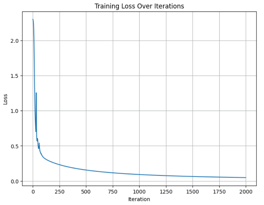
Step 7: Visualizing the Loss Curve
Plotting the loss gives us insight into the learning process:
plt.plot(losses)
plt.title("Training Loss Over Time")
plt.xlabel("Iteration")
plt.ylabel("Loss")
plt.grid(True)
plt.show()A smooth, downward-sloping curve means training is working as expected.
Step 8: Evaluating the Test Set
Let’s check how well our model performs on unseen data.
# 1: Compute the first linear transformation for the test data (input → hidden layer)
Z1_test = np.dot(X_test_flat, W1) + b1

# 2: Apply the ReLU activation to the hidden layer outputs
A1_test = relu(Z1_test)

# 3: Compute the second linear transformation (hidden → output layer)
Z2_test = np.dot(A1_test, W2) + b2

# 4: Apply the softmax activation to get class probabilities for each test sample
A2_test = softmax(Z2_test)

# 5: For each test sample, select the class (0–9) with the highest predicted probability
y_pred = np.argmax(A2_test, axis=1)

# 6: Compare predicted labels to the actual test labels and calculate accuracy
accuracy = np.mean(y_pred == y_test)

# 7: Print the final test accuracy as a percentage
print(f"Test Accuracy: {accuracy * 100:.2f}%")Final Test Accuracy: 97.47%
This is close to what you’d get with high-level libraries, and we built it all ourselves.
Step 9: Visualizing Predictions
Let’s pick some random digits from the test set and visualize how well the model did:
indices = np.random.choice(len(X_test_flat), 10, replace=False)

plt.figure(figsize=(15, 4))
for i, idx in enumerate(indices):
    image = X_test[idx].reshape(28, 28)
    true = y_test[idx]
    pred = y_pred[idx]
    color = 'green' if true == pred else 'red'
    plt.subplot(1, 10, i+1)
    plt.imshow(image, cmap='gray')
    plt.title(f"Pred: {pred}\nTrue: {true}", color=color)
    plt.axis('off')
plt.show()This step makes the model feel real. You can actually see what it got right and where it struggled.

Final Thoughts
This project taught me more about neural networks than any library could. By building it from scratch, I learned:
- How each layer transforms the data.
- Why activations like ReLU and Softmax matter.
- How loss functions guide learning.
- How backpropagation calculates gradients.
- How weight updates lead to better predictions.
Want to See the Full Code?
Check out the GitHub repository here: GitHub Repository Link


