Heart disease is one of the leading causes of death around the world. Predicting the risk of heart failure early can help save lives. In this guide, we’ll build a Heart Failure Prediction model using SVM with Scikit-Learn. You’ll learn how to train, evaluate, and understand a Support Vector Machine (SVM) model using real medical data, all in simple steps that beginners can follow.
Machine learning models like SVM are powerful for binary classification problems, such as predicting whether a patient is likely to survive heart failure. While building SVM from scratch helps you understand the math, using Scikit-Learn allows you to apply the same logic faster and more efficiently. It also gives you access to tuning parameters and tools for evaluation.
In this project, we’ll explore a real-world dataset, clean it, prepare the features, and train an SVM classifier to predict patient outcomes. Along the way, you’ll see how each step connects, from loading the data to evaluating accuracy and visualizing results. By the end, you’ll know how to use SVM in Scikit-Learn confidently for your own classification projects.
Project Overview
This project focuses on predicting heart failure outcomes using the Heart Failure Clinical Records Dataset from Kaggle, a real-world dataset that contains health records of patients collected during follow-up visits. Each record includes several medical features such as age, blood pressure, serum creatinine, ejection fraction, and smoking status, among others.
Our goal is simple:
- To predict whether a patient is likely to survive (1) or not survive (0) based on their clinical data.
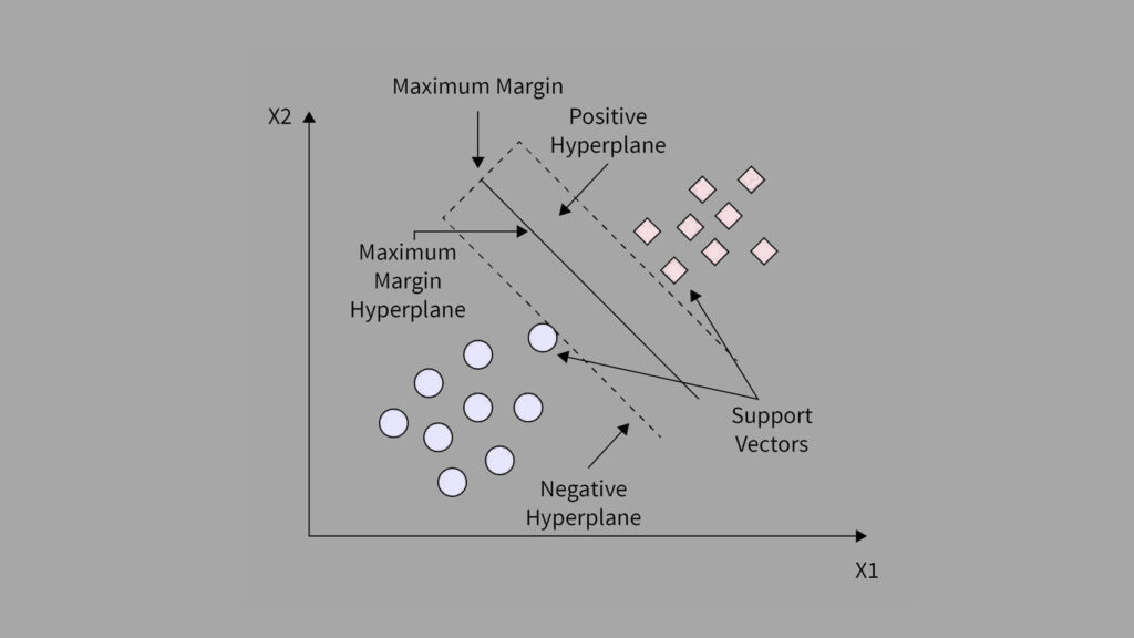
This makes it a binary classification problem, which is a perfect use case for Support Vector Machines (SVM).
SVM works by finding the best boundary that separates data points of different classes. In our case, it learns to separate patients who survived from those who did not, using combinations of their medical features.
Why Use SVM?
SVMs are known for their strong performance in high-dimensional spaces and their ability to handle both linear and nonlinear data. In medical prediction problems, relationships between variables are rarely simple. That’s why we use SVM with kernel functions (like RBF kernels) to map complex patterns in the data.
By the end of this project, you’ll understand how to:
- Load and explore a real-world medical dataset.
- Train and tune an SVM classifier using Scikit-Learn.
- Evaluate its performance using accuracy, precision, recall, and F1-score.
- Interpret the results visually for better understanding.
1. Importing Libraries and Loading the Dataset
Before we begin training our Support Vector Machine (SVM) model with Scikit-Learn, we first need to import the right tools.
In every machine learning project, we rely on a few essential Python libraries:
# Import core libraries
import pandas as pd
import numpy as np

# Import visualization tools
import matplotlib.pyplot as plt
import seaborn as sns

# Import machine learning tools
from sklearn.model_selection import train_test_split
from sklearn.preprocessing import StandardScaler
from sklearn.svm import LinearSVC
from sklearn.metrics import accuracy_score, f1_score, confusion_matrix, classification_report
from sklearn.model_selection import GridSearchCVWhat each library does:
- pandas: For reading, cleaning, and exploring data.
- numpy: For numerical calculations and handling arrays.
- matplotlib and seaborn: For data visualization. We use these to understand trends and relationships in the dataset.
- sklearn (Scikit-Learn): This is our main machine learning library. It provides tools for splitting data, scaling features, training models, and evaluating results.
2. Load and Preview Dataset
Next, we load our dataset, which contains medical records of heart failure patients.
# Load dataset
data = pd.read_csv('heart_failure_clinical_records_dataset.csv')

# Preview a few records
data.head()
- Each row here represents one patient’s clinical record, showing different health indicators measured during a medical study.
- Demographic and lifestyle details: Columns like
age,sex, andsmokinggive us background information about each patient. - Clinical features: Fields such as
ejection_fraction,serum_creatinine, andserum_sodiumhelp us understand how well the heart and kidneys are functioning. - Health conditions: Binary columns like
anaemia,diabetes, andhigh_blood_pressureindicate whether each condition is present (1) or absent (0). - Target variable: The last column,
DEATH_EVENT, tells us whether the patient died (1) or survived (0) during the follow-up period.
Next, we check the dataset’s structure using the info() function in pandas. This command shows the number of rows, columns, data types, and whether any values are missing.
# Data information structure
data.info()RangeIndex: 299 entries, 0 to 298
Data columns (total 13 columns):
# Column Non-Null Count Dtype
--- ------ -------------- -----
0 age 299 non-null float64
1 anaemia 299 non-null int64
2 creatinine_phosphokinase 299 non-null int64
3 diabetes 299 non-null int64
4 ejection_fraction 299 non-null int64
5 high_blood_pressure 299 non-null int64
6 platelets 299 non-null float64
7 serum_creatinine 299 non-null float64
8 serum_sodium 299 non-null int64
9 sex 299 non-null int64
10 smoking 299 non-null int64
11 time 299 non-null int64
12 DEATH_EVENT 299 non-null int64
dtypes: float64(3), int64(10)
- The dataset contains 299 patient records and 13 features in total.
- Every column has 299 non-null values, meaning there are no missing entries to clean up.
- Most features use the integer data type, representing binary or categorical information like
anaemia,diabetes, orhigh_blood_pressure. - A few columns such as
age,platelets,serum_creatinine, andserum_sodium— are continuous numerical variables that measure actual medical quantities.
This is good news because it means the data is complete and ready for analysis. We won’t need to fill or remove missing values, which keeps the preprocessing simple and clean.
To understand the range and behavior of each variable, we use the describe() function in pandas. It provides quick statistics such as the mean, standard deviation, and range for all numerical features.
# Statistical information
data.describe().T
- The average patient age is around 61 years, with most patients between 40 and 95 years old. This suggests that the dataset mainly focuses on older adults, the group most at risk for heart failure.
- The average ejection fraction (which measures how well the heart pumps blood) is about 38%. Healthy hearts usually pump at 50–70%, so many patients in this dataset have weakened heart function.
- Serum creatinine values, ranging from 0.5 to 9.4 mg/dL, show a wide variation in kidney function among patients.
- The creatinine phosphokinase (CPK) levels vary greatly, from 23 to 7861, suggesting that some patients experienced acute muscle or heart injury.
- The serum sodium levels are mostly between 134 and 140, which falls within a typical clinical range.
In summary, the data looks numerically consistent and reflects realistic clinical variations seen in patients with heart failure. This gives us confidence that the dataset is reliable for model training.
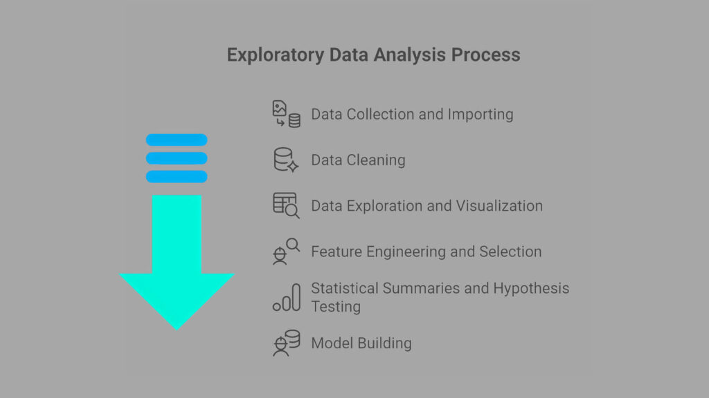
3. Exploratory Data Analysis (EDA)
Before diving into model training, it’s crucial to first explore and understand the dataset. EDA helps reveal both statistical trends and clinical patterns that could influence patient outcomes.
By systematically analyzing the data, we can spot potential issues, uncover relationships between features, and form initial hypotheses about what factors might predict heart failure mortality.
In this stage, our goals are to:
- Visualize survival patterns – Observe how certain features differ between patients who survived and those who didn’t.
- Understand feature distributions – Explore how clinical measurements like age, ejection fraction, and serum creatinine vary across patients.
- Check class balance – Assess whether the dataset has a balanced number of survivors and deaths, which is key for fair model learning.
- Analyze correlations – Identify meaningful relationships between features, such as how kidney function might relate to heart performance.
3.1. Distribution of the Target Variable (DEATH_EVENT)
Let’s start by examining the target variable, DEATH_EVENT, which indicates whether a patient survived (0) or died (1) during the follow-up period.
The distribution is visualized below:
# Plot the target distribution
sns.countplot(data=data, x='DEATH_EVENT', palette='Set2')
plt.title('Distribution of Target (DEATH_EVENT)')
plt.xlabel('DEATH_EVENT: survived (0) or died (1)')
plt.ylabel('Count')
plt.show()
To quantify the counts and proportions:
# Calculate classes count
data['DEATH_EVENT'].value_counts().to_frame(name='Count').assign(
Percent=lambda x: round((x['Count'] / x['Count'].sum()) * 100, 2))Count Percent
DEATH_EVENT
0 203 67.89
1 96 32.11
Insights
- 203 patients (≈ 68%) survived.
- 96 patients (≈ 32%) passed away.
This reveals a moderately imbalanced dataset, with more survivors than deaths. While the imbalance isn’t severe, it’s still important to consider because Support Vector Machines can be sensitive to class imbalance.
To ensure fair model learning later, we’ll apply techniques such as class weighting (e.g., class_weight='balanced') during model training.
3.2 Univariate Analysis of Features
Now that we’ve explored the target variable, let’s take a closer look at how each individual feature behaves. This process helps us understand the distribution, range, and potential clinical relevance of each variable before examining relationships between them.
We’ll analyze both continuous and categorical variables:
- Continuous features:
age,ejection_fraction,serum_creatinine,serum_sodium,platelets,creatinine_phosphokinase, andtime. - Categorical features:
anaemia,diabetes,high_blood_pressure,sex, andsmoking.
Understanding these patterns provides a foundation for later identifying risk factors, detecting outliers, and preparing the data for modeling.
3.2.1 Categorical Features Analysis
We begin with categorical (binary) clinical variables. Factors that describe the presence or absence of specific health conditions or habits.
desc_dict = {
    'anaemia': ('non-anaemic', 'anaemic'),
    'diabetes': ('non-diabetic', 'diabetic'),
    'high_blood_pressure': ('non-hypertensive', 'hypertensive'),
    'sex': ('female', 'male'),
    'smoking': ('non-smoker', 'smoker'),
}

# Plot distribution of categorical features
plt.figure(figsize=(18, 10))
for i, col in enumerate(categorical_feat, 1):
    plt.subplot(2, 3, i)
    sns.countplot(data=data, x=col, palette='Set2')
    plt.title(f'Distribution of {col}')
    plt.xlabel(f'{col}: {desc_dict[col][0]} (0) or {desc_dict[col][1]} (1)')
    plt.ylabel('Count')
plt.subplots_adjust(hspace=0.4)
plt.show()
To quantify the counts and proportions:
# Calculate classes count
for col in categorical_feat:
    count = data[col].value_counts().to_frame(name='Count').assign(
        Percent=lambda x: round((x['Count'] / x['Count'].sum()) * 100, 2))
    print(f'=== {col} ===')
    print(count)
=== high_blood_pressure ===
                     Count  Percent
high_blood_pressure
0                      194    64.88
1                      105    35.12

=== anaemia ===
         Count  Percent
anaemia
0          170    56.86
1          129    43.14

=== diabetes ===
          Count  Percent
diabetes
0           174    58.19
1           125    41.81
=== sex ===
     Count  Percent
sex
1      194    64.88
0      105    35.12

=== smoking ===
         Count  Percent
smoking
0          203    67.89
1           96    32.11
From these distributions, we can draw several observations about the study population:
- Most patients are male, non-smokers, and non-hypertensive.
- Despite that, a substantial proportion suffer from conditions such as anaemia and diabetes, both of which are associated with worse heart outcomes.
- The variety of health conditions captured here provides a rich dataset for identifying patterns and predictors of mortality in heart failure patients.
In the next section, we’ll explore continuous features such as age, ejection fraction, and serum measurements to uncover deeper numerical trends and potential outliers.
3.2.2 Continuous Features Analysis
After examining the categorical variables, let’s now explore the continuous clinical features to understand their statistical properties and detect any irregularities such as skewness or outliers.
These features, like age, ejection fraction, and serum creatinine, often provide the most crucial physiological insights into patient health.
We visualized each feature using histograms and boxplots to capture both their distribution shape and the presence of potential outliers.
# Plot distribution of categorical features
for col in continuous_feat:
    plt.figure(figsize=(12, 4))

    # Histogram
    plt.subplot(1, 2, 1)
    sns.histplot(data=data, x=col, kde=True, color='lightblue')
    plt.title(f'Distribution of {col}')
    plt.xlabel(col)
    plt.ylabel('Count')

    # Boxplot
    plt.subplot(1, 2, 2)
    sns.boxplot(data=data, y=col, color='lightblue')
    plt.title(f'Boxplot of {col}')
    plt.ylabel(col)

    if col in ['creatinine_phosphokinase', 'platelets']:
        plt.yticks(rotation=45)

plt.tight_layout()
plt.show()


We then computed the skewness and number of outliers for each feature to quantify how symmetric or skewed the distributions are:
# Checking for skew and outliers
for col in continuous_feat:
    q1 = data[col].quantile(0.25)
    q3 = data[col].quantile(0.75)
    iqr = q3 - q1
    lower = q1 - iqr * 1.5
    upper = q3 + iqr * 1.5
    outliers = data[(data[col] < lower) | (data[col] > upper)][col]
    print(f'=== {col} ===')
    print("Outliers:", len(outliers))
print("Skew:", data[col].skew())=== age === Outliers: 0 Skew: 0.42306190672863536 === creatinine_phosphokinase === Outliers: 29 Skew: 4.463110084653752 === ejection_fraction === Outliers: 2 Skew: 0.5553827516973211 === time === Outliers: 0 Skew: 0.12780264559841184
=== platelets ===
Outliers: 21
Skew: 1.4623208382757793

=== serum_creatinine ===
Outliers: 29
Skew: 4.455995882049026

=== serum_sodium ===
Outliers: 4
Skew: -1.0481360160574988
From the above analysis, several trends stand out:
- Most physiological measures like age, ejection fraction, and follow-up time are roughly symmetric, indicating a well-distributed dataset for these parameters.
- In contrast, creatinine phosphokinase (CPK) and serum creatinine show strong positive skewness, reflecting that a small number of patients experienced extreme clinical values. These may correspond to cases of acute heart damage or renal dysfunction.
- Platelet counts also display mild skewness, while serum sodium trends slightly negative, meaning lower sodium levels occur less frequently but could be clinically significant.
- Overall, the dataset presents long-tailed distributions and real-world variability typical of medical data.
Such features often require scaling or log transformations during preprocessing to ensure stable model performance particularly for algorithms like SVM, which are sensitive to feature magnitude.
3.3 Bivariate Analysis of Features vs Target (DEATH_EVENT)
After understanding each feature individually, the next step is to explore how they relate to the target variable, DEATH_EVENT, which indicates whether a patient survived (0) or died (1) during the follow-up period.
This bivariate analysis helps uncover which patient characteristics are most associated with mortality and which have weaker or negligible effects. We will analyze both categorical and continuous features to gain a holistic view of the data.
3.3.1 Categorical Features vs Target
To examine how categorical features relate to survival outcomes, we compared the average proportion of each category between survivors and non-survivors using bar plots and group-wise means.
plt.figure(figsize=(18, 10))
for i, col in enumerate(categorical_feat, 1):
    plt.subplot(2, 3, i)
    sns.barplot(data=data, y=col, hue='DEATH_EVENT', ci=False, palette='Set2', estimator='mean')
    plt.title(f'Distribution of {col} vs DEATH_EVENT')
    plt.xlabel('DEATH_EVENT: survived (0) or died (1)')
    plt.ylabel(col)
plt.subplots_adjust(hspace=0.3)
plt.show()
To quantify the counts, let’s look at some statistics:
category_feat_mean = data.groupby('DEATH_EVENT')[categorical_feat].mean().T
round(category_feat_mean, 2)DEATH_EVENT 0 1
anaemia 0.41 0.48
diabetes 0.42 0.42
high_blood_pressure 0.33 0.41
sex 0.65 0.65
smoking 0.33 0.31
From these results, we can observe:
- Anaemia and high blood pressure appear to be mild predictors of mortality, likely due to their roles in oxygen supply and cardiovascular strain.
- Diabetes, surprisingly, does not show a strong direct association with death in this dataset, though it may influence other risk factors indirectly.
- Sex and smoking seem largely neutral in determining survival outcomes, though these findings should be interpreted cautiously due to the moderate dataset size.
Overall, these categorical comparisons suggest that clinical conditions directly affecting heart or blood function (like anaemia and hypertension) are more indicative of mortality risk than lifestyle or demographic variables.
3.3.2. Continuous Features vs Target (DEATH_EVENT) Analysis
After exploring categorical features, the next step is to examine how continuous variables differ between patients who survived (0) and those who died (1). This analysis helps reveal which physiological measurements may be strong indicators of heart failure risk.
To do this, we will visualize each continuous feature against the target variable using boxplots, and then summarize their statistical properties, mean, median, quartiles, and spread across both outcome groups.
plt.figure(figsize=(18, 12))
for i, col in enumerate(continuous_feat, 1):
    plt.subplot(3, 3, i)
    sns.boxplot(data=data, x='DEATH_EVENT', y=col, palette='Set2')
    plt.title(f'{col} vs DEATH_EVENT')
    plt.xlabel('DEATH_EVENT: survived (0) or died (1)')
    plt.ylabel(col)
plt.show()
Let’s look at some statistics:
for col in continuous_feat:
    col_mean = data.groupby('DEATH_EVENT')[col].describe().T
    print(f'=== {col} vs DEATH_EVENT ===')
print(round(col_mean, 2))=== age vs DEATH_EVENT === DEATH_EVENT 0 1 count 203.00 96.00 mean 58.76 65.22 std 10.64 13.21 min 40.00 42.00 25% 50.00 55.00 50% 60.00 65.00 75% 65.00 75.00 max 90.00 95.00 === creatinine_phosphokinase vs DEATH_EVENT === DEATH_EVENT 0 1 count 203.00 96.00 mean 540.05 670.20 std 753.80 1316.58 min 30.00 23.00 25% 109.00 128.75 50% 245.00 259.00 75% 582.00 582.00 max 5209.00 7861.00 === ejection_fraction vs DEATH_EVENT === DEATH_EVENT 0 1 count 203.00 96.00 mean 40.27 33.47 std 10.86 12.53 min 17.00 14.00 25% 35.00 25.00 50% 38.00 30.00 75% 45.00 38.00 max 80.00 70.00 === platelets vs DEATH_EVENT === DEATH_EVENT 0 1 count 203.00 96.00 mean 266657.49 256381.04 std 97531.20 98525.68 min 25100.00 47000.00 25% 219500.00 197500.00 50% 263000.00 258500.00 75% 302000.00 311000.00 max 850000.00 621000.00
=== serum_creatinine vs DEATH_EVENT ===
DEATH_EVENT       0      1
count        203.00  96.00
mean           1.18   1.84
std            0.65   1.47
min            0.50   0.60
25%            0.90   1.08
50%            1.00   1.30
75%            1.20   1.90
max            6.10   9.40

=== serum_sodium vs DEATH_EVENT ===
DEATH_EVENT       0       1
count        203.00   96.00
mean         137.22  135.38
std            3.98    5.00
min          113.00  116.00
25%          135.50  133.00
50%          137.00  135.50
75%          140.00  138.25
max          148.00  146.00

=== time vs DEATH_EVENT ===
DEATH_EVENT       0       1
count        203.00   96.00
mean         158.34   70.89
std           67.74   62.38
min           12.00    4.00
25%           95.00   25.50
50%          172.00   44.50
75%          213.00  102.25
max          285.00  241.00
- Age, ejection fraction, and serum creatinine emerge as key clinical indicators of survival.
- Features like CPK and serum sodium show high variability, hinting at the need for robust preprocessing and possibly transformation before modeling.
- The presence of outliers in certain features (e.g., CPK and creatinine) underscores the biological diversity within the patient group and signals that normalization or scaling will be important in later steps.
By combining statistical summaries with visual inspection, we can better understand the underlying clinical patterns in this dataset and prepare for effective feature engineering and predictive modeling.
3.4 Collinearity and Multicollinearity Analysis
Understanding how features relate to one another is an essential part of exploratory data analysis. Highly correlated variables can introduce multicollinearity, which can distort model interpretations, especially in algorithms that rely on coefficient estimates (like logistic regression or linear models).
To assess this, we will compute the correlation matrix for all numerical variables and visualize it using a heatmap.
# Collinearity of variables
corr_mat = data.corr()
plt.figure(figsize=(18, 12))
sns.heatmap(corr_mat, cmap='coolwarm', annot=True, linewidths=0.5)
plt.title("Variable Collinearity")
plt.show()
- Age: There is a moderate positive correlation of approximately +0.25 with
DEATH_EVENT. This means that older patients tend to have a higher likelihood of mortality compared to younger ones. - Ejection Fraction: This feature shows a moderate negative correlation of about –0.27 with
DEATH_EVENT. A lower ejection fraction, which reflects weaker pumping efficiency of the heart, is strongly associated with a higher risk of death. - Serum Creatinine: The correlation with
DEATH_EVENTis around +0.29, indicating that higher creatinine levels (signifying impaired kidney function) are linked to increased mortality risk. - Time: This variable has a relatively strong negative correlation of –0.53 with
DEATH_EVENT. In other words, patients who lived longer had longer follow-up times, while those who died earlier naturally had shorter follow-up durations.
Overall, these observations suggest that age, cardiac efficiency (ejection fraction), kidney function (serum creatinine), and follow-up time are among the most influential factors affecting patient survival.
4. Implementing SVM with Scikit-Learn
In this section, we’ll implement and optimize an SVM with Scikit-Learn to predict patient mortality based on the Heart Failure dataset. Our approach integrates data preprocessing, model training, hyperparameter tuning, and evaluation to achieve a reliable predictive model.
Step 1: Data Preparation and Splitting
We begin by separating the features (X) from the target variable (y = DEATH_EVENT). The dataset is then divided into training and testing subsets using an 80/20 split, ensuring stratification to maintain class balance.
To standardize feature scaling which is crucial for SVMs due to their sensitivity to feature magnitudes, we use a StandardScaler inside a Scikit-Learn Pipeline. This ensures a clean and reproducible workflow.
# Separate features and target variable
X = data.drop(columns=['DEATH_EVENT'])
y = data['DEATH_EVENT']

# Split the dataset into training and testing sets
X_train, X_test, y_train, y_test = train_test_split(
    X, y, test_size=0.2, stratify=y, random_state=42
)Step 2: Building the SVM Model and Hyperparameter Tuning
We implement a Linear Support Vector Classifier (LinearSVC) within a pipeline and perform GridSearchCV to fine-tune hyperparameters.
The grid search explores different values of the regularization parameter C, while keeping the penalty fixed at 'l2' and loss as 'squared_hinge'.
# Create a pipeline with StandardScaler + LinearSVC
pipeline = Pipeline([
    ("scaler", StandardScaler()),
    ("svm", LinearSVC(max_iter=5000, random_state=42))]
)

# Define hyperparameter grid for tuning
param_grid = {
    "svm__C": [0.001, 0.01, 0.1, 1, 10],
    "svm__penalty": ["l2"],
    "svm__loss": ["squared_hinge"]
}

# Set up GridSearchCV for hyperparameter tuning
grid_search = GridSearchCV(
    estimator=pipeline,
    param_grid=param_grid,
    cv=5,
    scoring='accuracy',
    n_jobs=-1,
    verbose=2
)

# Fit the grid search on the scaled training data
grid_search.fit(X_train, y_train)

# Display the best combination of hyperparameters and corresponding accuracy
print("Best parameters found:", grid_search.best_params_)
print("Best cross-validation accuracy:", grid_search.best_score_)Fitting 5 folds for each of 5 candidates, totalling 25 fits
Best parameters found: {'svm__C': 0.001, 'svm__loss': 'squared_hinge', 'svm__penalty': 'l2'}
Best cross-validation accuracy: 0.8367021276595745
This configuration achieved a cross-validation accuracy of approximately 83.67%, indicating a strong baseline generalization.
Step 3: Model Evaluation on Test Data
We will evaluate the optimized model on the test set to assess its real-world performance.
# Retrieve the best SVM model from the grid search
best_svm = grid_search.best_estimator_

# Make predictions on the scaled test set
y_pred = best_svm.predict(X_test)

# Evaluate model performance on test data
print("Accuracy:", accuracy_score(y_test, y_pred))
print("F1 Score:", f1_score(y_test, y_pred))
print("Confusion Matrix:\n", confusion_matrix(y_test, y_pred))
print("Classification Report:\n", classification_report(y_test, y_pred))Accuracy: 0.8166666666666667
F1 Score: 0.6451612903225806
Confusion Matrix:
[[39 2]
[9 10]]
Classification Report:
precision recall f1-score support
0 0.81 0.95 0.88 41
1 0.83 0.53 0.65 19
accuracy 0.82 60
macro avg 0.82 0.74 0.76 60
weighted avg 0.82 0.82 0.80 60
- Accuracy: The model achieved an accuracy of 82%, meaning it correctly classified 82% of all patient outcomes.
- F1 Score: The F1 score was 0.65, which balances precision and recall and reflects a good trade-off between the two.
- Precision (Death class): Precision for predicting death cases was 0.83, showing that when the model predicts a patient will die, it’s correct 83% of the time.
- Recall (Death class): The recall was 0.53, meaning the model correctly identified 53% of actual death cases.
In summary, the SVM model with Scikit-learn demonstrates strong precision and overall accuracy but leaves some room for improvement in recall, indicating that while it’s confident in its positive predictions, it may miss some true death cases.
This balance makes it a solid starting point for medical outcome prediction, where precision often carries high importance.
5. Conclusion
In this project, we explored how to build, train, and evaluate an SVM with Scikit-learn to predict mortality among heart failure patients. Starting from exploratory data analysis (EDA) and feature relationships to model training and evaluation, each step demonstrated the power and practicality of SVMs in real-world healthcare data applications.
By leveraging Scikit-learn’s LinearSVC class, we were able to:
- Efficiently handle both categorical and continuous data.
- Use kernel-based learning to capture complex, non-linear patterns.
- Evaluate performance using metrics like accuracy, precision, recall, and F1-score for a well-rounded view of model effectiveness.
Our SVM model achieved an accuracy of 82%, indicating strong overall performance in distinguishing between patients who survived and those who did not. While recall was relatively lower than precision, this result is typical for imbalanced medical datasets where false negatives can be challenging to minimize.
This project highlights how SVM with Scikit-learn can be a robust choice for medical classification problems, offering solid generalization, interpretability through kernel selection, and strong predictive capabilities with limited parameter tuning. In future work, the model can be further enhanced using:
- Hyperparameter optimization (via GridSearchCV).
- Feature scaling and selection for improved stability.
- Model comparison with tree-based ensembles or neural networks.
Ultimately, this project not only reinforced the theoretical foundations of SVMs but also provided hands-on experience in applying them to a meaningful, real-world problem. It serves as an excellent example of how Scikit-learn simplifies the implementation of powerful machine learning algorithms in Python.